1   Exam 1 answers

are now online.

We gave full points even if you didn't finish the arithmetic to compute a number. In the real world, you have computers. Also, in the real world, accurate analysis and computation matter. In 1954, physicists made an eensy teensy error designing Castle Bravo.

2   Homework 6

online, due in one week (i.e., Thurs).

3   Notation

How to parse $F_X(x)$

1. Uppercase F means that this is a cdf. Different letters may indicate different distributions.
2. The subscript X is the name of the random variable.
3. The x is an argument, i.e., an input.
4. $F_X(x)$ returns the probability that the random variable is less or equal to the value x, i.e. prob(X<=x).

4   Matlab

1. Matlab

   1. Major functions:

      cdf(dist,X,A,...)
      pdf(dist,X,A,...)
      

   2. Common cases of dist (there are many others):

      'Binomial'
      'Exponential'
      'Poisson'
      'Normal'
      'Geometric'
      'Uniform'
      'Discrete Uniform'
      

   3. Examples:

      pdf('Normal',-2:2,0,1)
      cdf('Normal',-2:2,0,1)
      
      p=0.2
      n=10
      k=0:10
      bp=pdf('Binomial',k,n,p)
      bar(k,bp)
      grid on
      
      bc=cdf('Binomial',k,n,p)
      bar(k,bc)
      grid on
      
      x=-3:.2:3
      np=pdf('Normal',x,0,1)
      plot(x,np)
      

   4. Interactive GUI to explore distributions: disttool

   5. Random numbers:

      rand(3)
      rand(1,5)
      randn(1,10)
      randn(1,10)*100+500
      randi(100,4)
      

   6. Interactive GUI to explore random numbers: randtool

   7. Plotting two things at once:

      x=-3:.2:3
      n1=pdf('Normal',x,0,1)
      n2=pdf('Normal',x,0,2)
      plot(x,n1,n2)
      plot(x,n1,x,n2)
      plot(x,n1,'--r',x,n2,'.g')
      

2. Use Matlab to compute a geometric pdf w/o using the builtin function.

5   Text ctd

1. Section 4.2.1 page 150.

6   Material added after class

1. My handwritten tablet notes.

How to submit

Submit to LMS; see details in syllabus.

Questions

All questions are from the text.

Each part of a question is worth 5 points.

1. 4.5 on page 215.
2. 4.8 on page 216.
3. 4.17 on page 217.
4. 4.33 on page 218.

Total: 55 pts.

1   The different counting formulae for selecting k items from n

1. With replacement; order matters: \(n^k\).
2. W/o replacement; order matters: \(n(n-1)\cdots(n-k+1) = \frac{n!}{(n-k)!}\).
3. With replacement; order does not matter: \({{n-1+k} \choose k}\)
4. W/o replacement; order does not matter: \({n\choose k}=\frac{n!}{k!(n-k)!}\).

2   Review questions

1. Sampling with replacement with ordering: Each day I eat lunch at either the Union, Mcdonalds, Brueggers, or Sage. How many ways can I eat lunch over 5 days next week?
2. sampling w/o replacement and w/o order: How many different possible teams of 3 people can you pick from a group of 5?
3. sampling w/o replacement and with order: 5 people run a race for gold, silver, bronze. How many ways can the medals be won, w/o any ties?
4. binomial: A coin falls heads with p=.6. You toss it 3 times. What's the probability of 2 heads and 1 tail?
5. multinomial: You play 38-slot roulette 3 times. Once you got red, once black and once 0 or 00. What was the probability?
6. conditional probability: You have 2 dice, one 6-sided and one 12-sided. You pick one of them at random and throw it w/o looking; the top is 2. What's the probability that you threw the 6-sided die?
7. What's the expected number of times you'll have to toss the unknown die to get your first 2?
8. Independence: Consider {1,2,3,...12}. Is the set of even numbers independent of the set of multiples of 3? What if we use {1,2,..10}?
9. Useful review questions from the text.
   1. 2.83 on page 90.
   2. 2.99.
   3. 3.5 on page 130.
   4. 3.9.
   5. 3.15.
   6. 3.26.
   7. 3.88 on page 139.

3   Iclicker

1. We often add a check bit to an 8-bit byte, and set it so there are an odd number of 1 bits. When we read the byte, which is now 9 bits, if there are an even number of 1 s, then we know that there was an error.

   Assume that the probability of any one bit going bad is 1e-10. (The real number is much smaller.)

   What is the probability of the byte going bad (within 1 significant digit)?

   1. 1e-10
   2. 8e-10
   3. 9e-10
   4. 3.6e-19
   5. 7.2e-19

2. What is the probability of the byte going bad, but we don't notice that (because there were 2 bad bits)?

   1. 1e-10
   2. 8e-10
   3. 9e-10
   4. 3.6e-19
   5. 7.2e-19

4   Chapter 4 ctd

1. Taxi example: Sometimes there are mixed discrete and continuous r.v.
   1. Let X be the time X to get a taxi at the airport.
   2. 80% of the time a taxi is already there, so p(X=0)=.8.
   3. Otherwise we wait a uniform time from 0 to 20 minutes, so p(a<x<b)=.01(b-a), for 0<a<b<20.
2. Iclicker. For the taxi example, what is F(0)?
   1. 0
   2. .2
   3. .8
   4. .81
   5. 1
3. iclicker. For the taxi example, what is F(1)?
   1. 0
   2. .8
   3. .81
   4. .9
   5. 1
4. Simple continuous r.v. examples: uniform, exponential.
5. The exponential distribution complements the Poisson distribution. The Poisson describes the number of arrivals per unit time. The exponential describes the distribution of the times between consecutive arrivals.
6. The most common continuous distribution is the normal distribution.
7. Conditional probabilities work the same with continuous distributions as with discrete distributions.
8. Using Matlab: Matlab, Mathematica, and Maple all will help you do problems too big to do by hand. I'll demo Matlab since IMO more of the class knows it.
9. Iclicker. Which of the following do you prefer to use?
   1. Matlab
   2. Maple
   3. Mathematica
   4. Paper. It was good enough for Bernoulli and Gauss; it's good enough for me.
   5. Something else (please email about it me after the class).

5   Material added after class

1. My handwritten tablet notes.

1   Iclicker questions

What is the best discrete probability distribution in the following cases.

1. Your car has five tires (including the spare), which may each independently be flat. The event is that not more than one tire is flat.
   1. Bernoulli
   2. binomial
   3. geometric
   4. Poisson
   5. uniform
2. 1,000,000 widgets are made this year, of which 1,000 are bad. You buy 5 at random. The event is that not more than one widget is bad.
   1. Bernoulli
   2. binomial
   3. geometric
   4. Poisson
   5. uniform
3. You toss a weighted coin, which lands heads 3/4 of the time.
   1. Bernoulli
   2. binomial
   3. geometric
   4. Poisson
   5. uniform
4. You toss a fair 12-sided die.
   1. Bernoulli
   2. binomial
   3. geometric
   4. Poisson
   5. uniform
5. You're learning to drive a car, and trying to pass the test. The event of interest is the number of times you have to take the test to pass. Assume that the tests are independent of each other and have equal probability.
   1. Bernoulli
   2. binomial
   3. geometric
   4. Poisson
   5. uniform
6. It's Nov 17 and you're outside in a dark place looking for Leonid meteorites. The event of interest is the number of meteorites per hour that you see.
   1. Bernoulli
   2. binomial
   3. geometric
   4. Poisson
   5. uniform
7. It's Nov 17.... The new event of interest is the number of seconds until you see the next meteorite.
   1. Bernoulli
   2. binomial
   3. geometric
   4. Poisson
   5. uniform

2   Exam 1

1. Closed book but a calculator and one 2-sided letter-paper-size note sheet is allowed.
2. Material is from chapters 1-3.
3. Questions will be based on book, class, and homework, examples and exercises.
4. The hard part for you may be deciding what formula to use.
5. Any calculations will (IMHO) be easy.
6. Speed should not be a problem; most people should finish in 1/2 the time.

3   Chapter 3 exercises

We'll try these exercises from the text in class.

1. 3.51a in page 135.
2. 3.39 on page 139.
3. 3.91.

4   Chapter 4

1. I will try to ignore most of the theory at the start of the chapter.
2. Now we will see continuous random variables.
   1. The probability of the r.v being any exact value is infinitesimal,
   2. so we talk about the probability that it's in a range.
3. Sometimes there are mixed discrete and continuous r.v.
   1. Let X be the time X to get a taxi at the airport.
   2. 80% of the time a taxi is already there, so p(X=0)=.8.
   3. Otherwise we wait a uniform time from 0 to 20 minutes, so p(a<x<b)=.01(b-a), for 0<a<b<20.
4. Remember that for discrete r.v. we have a probability mass function (pmf).
5. For continuous r.v. we now have a probability density function (pdf), \(f_X(x)\).
6. p(a<x<a+da) = f(a)da
7. For any r.v., we have a cumulative distribution function (cdf) \(F_X(x)\).
8. The subscript is interesting only when we are using more than one cdf and need to tell them apart.
9. Definition: F(x) = P(X<=x).
10. The <= is relevant only for discrete r.v.
11. As usual Wikipedia isn't bad, and is deeper than we need here, Cumulative_distribution_function.
12. We compute means and other moments by the obvious integrals.

5   Material added after class

1. My handwritten tablet notes.

How to submit

Submit to LMS; see details in syllabus.

Questions

All questions are from the text.

Each part of a question is worth 5 points.

1. 3.11a and b on page 131.
2. 3.35 a-d on page 133.
3. 3.53 a and b on p 135.
4. 3.88 a-c on p 139.
5. 3.90 on p 139.

Total: 60 pts.

1   Homework 1-3 solutions

1. https://docs.google.com/document/d/1TPQIZpP6F4TbZZy4aU_damf5eEy8F4vQx0KOS3yP7NU/edit?usp=sharing
2. https://docs.google.com/document/d/1rt3ahzZy-wYaycr3ZCts2UHI7Ik68X3QJjtZxCTVva8/edit?usp=sharing
3. https://docs.google.com/document/d/1mMLkUCW4lLvNj7UeWRlKWP906V7hxgr0-Wg1ySM9Ncw/edit?usp=sharing

2   Chapter 3 ctd

1. Example 3.22 Variance of geometric r.v. We'll derive it.

2. Example 3.24 Residual waiting time

   1. X, time to xmit message, is uniform in 1...L.
   2. If X is over m, what's probability that remaining time is j?
   3. \(p_X(m+j|X>m) = \frac{P[X =m+j]}{P[X>m]} = \frac{1/L}{(L-m)/L} = 1/(L-m)\)

3. \(p_X(x) = \sum p_X(x|B_i) P[B_i]\)

4. Example 3.25 p 113 device lifetimes

   1. 2 classes of devices, geometric lifetimes.
   2. Type 1, probability \(\alpha\), parameter r. Type 2 parameter s.
   3. What's pmf of the total set of devices?

5. Example 3.26.

6. 3.5 More important discrete r.v

7. Table 3.1: We haven't seen \(G_X(z)\) yet.

8. 3.5.4 Poisson r.v.

   1. The experiment is observing how many of a large number of rare events happen in, say, 1 minute.

   2. E.g., how many cosmic particles hit your DRAM, how many people call to call center.

   3. The individual events are independent.

   4. The r.v. is the number that happen in that period.

   5. There is one parameter, \(\alpha\). Often this is called \(\lambda\).

      \begin{equation*} p(k) = \frac{\alpha^k}{k!}e^{-\alpha} \end{equation*}

   6. Mean and std dev are both \(\alpha\).

   7. In the real world, events might be dependent.

3   Material added after class

1. My handwritten tablet notes.

How to submit

Submit to LMS; see details in syllabus.

Questions

1. (5 points) This is a followup on last week's first question, which was this:

   Assume that it is known that one person in a group of 100 committed a crime. You're in the group, so there's a prior probability of 1/100 that you are it. There is a pretty good forensic test. It makes errors (either way) only 0.1% of the time. You are given the test; the result is positive. Using this positive test, what's the probability now that you are the criminal? (Use Bayes.)

   With a lot of tests, the results are grey, and the person running them has a choice in how to interpret them: lean towards finding someone guilty (but falsely accusing an innocent person), or the other way toward finding someone innocent (but letting a guilty person go free).

   Assume that in this example, the administrator can choose the bias. However the sum of the two types of errors is constant at 0.2%. (Whether that relation is really true would depend on the test.)

   This question is to plot both the number of innocent people falsely found guilty and the number of guilty people wrongly let go, as a function of the false positive rate. Use any plot package. Both numbers of people will usually be fractional.

2. (5 pts) Do exercise 2.126, page 95.

3. (5 pts) Do exercise 2.127.

4. (5 pts) Do exercise 3.1 on page 130.

5. (5 pts) Do exercise 3.5.

6. (5 pts) Do exercise 3.13 on page 132.

7. (5 pts) Do exercise 3.15.

Total: 35 pts.

1   Office hours and TAs

1. There are 2 grad TAs:

   1. Yi Fan fany4ATrpi.edu
   2. Amelia Peterson petera7ATrpi.edu

   and one undergrad:

   1. Jieyu Chen chenj35ATrpi.edu

   replace AT with (you figure it out).

2. Jieyu has taken this course, although from a different prof. She will prepare homework solutions.

3. Yi and Amelia will grade.

4. All three will hold office hours:

   1. Jieyu Chen: Fri 2:30 in the ECSE Flip Flop lounge, JEC6037.
   2. Amelia Peterson: Wed 12-2 in the Flip Flop lounge.
   3. Yi Fan: Tue 3-5, on the third floor of the library, in the open area near the window.

   Any changes will be pre-announced.

   Go towards the start of the time, otherwise they may leave.

   OTOH, if you need more time, or another time, write them. The goal is that every student who wants personal time will get it. (Want to talk with me after class over coffee; ok.)

5. Between the lectures, where I stay after class to answer questions, and their office hours, you have someone available 5 days a week.

2   Wikipedia

Wikipedia's articles on technical subjects can be excellent. In fact, they often have more detail than you want. Here are some that are relevant to this course. Read at least the first few paragraphs.

1. https://en.wikipedia.org/wiki/Outcome_(probability)
2. https://en.wikipedia.org/wiki/Random_variable
3. https://en.wikipedia.org/wiki/Indicator_function
4. https://en.wikipedia.org/wiki/Gambler%27s_fallacy
5. https://en.wikipedia.org/wiki/Fat-tailed_distribution

Nevertheless, Wikipedia can have errors, or at least definition differences from our text. E.g., https://en.wikipedia.org/wiki/Outcome_(probability) says that a discrete probability distribition has a finite sample space. Wrong, it could be countably infinite.

3   Independence of 3 random variables

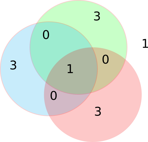
There was a question last week. If 3 r.v. are independent, does that mean that pairs of them are independent? The answer is no. See this Venn diagram:

1. Let R,G,B mean red, green, blue.
2. P(R) = P(B) = P(G) = 1/2
3. P(R and G and B) = 1/8 = P(R) P(B) P(G) so the triple is independent.
4. P(R and G) = 0 != P(R) P(G) so the pair are not independent.
5. You have to test every subset for independence.
6. Wikipedia also talks about this.

4   Two types of testing errors

1. There's an event A, with probability P[A]=p.
2. There's a dependent event, perhaps a test or a transmission, B.
3. You know P[B|A] and P[B|A'].
4. Wikipedia:
   1. https://en.wikipedia.org/wiki/Type_I_and_type_II_errors
   2. https://en.wikipedia.org/wiki/Sensitivity_and_specificity
5. Terminology:
   1. Type I error, False negative.
   2. Type II error, false positive.
   3. Sensitivity, true positive proportion.
   4. Selectivity, true negative proportion.

5   Chapter 3 ctd

1. This chapter covers Discrete (finite or countably infinite) r.v.. This contrasts to continuous, to be covered later.

2. Discrete r.v.s we've seen so far:

   1. uniform: M events 0...M-1 with equal probs
   2. bernoulli: events: 0 w.p. q=(1-p) or 1 w.p. p
   3. binomial: # heads in n bernoulli events
   4. geometric: # trials until success, each trial has probability p.

3. 3.1.1 Expected value of a function of a r.v.

   1. Z=g(X)
   2. E[Z] = E[g(x)] = \(\sum_k g(x_k) p_X(x_k)\)

4. Example 3.17 square law device

5. \(E[a g(X)+b h(X)+c] = a E[g(X)] + b E[h(x)] + c\)

6. Example 3.18 Square law device continued

7. Example 3.19 Multiplexor discards packets

8. Compute mean of a binomial distribution (started last Fri).

9. Compute mean of a geometric distribution (started last Fri).

10. 3.3.1, page 107: Operations on means: sums, scaling, functions

11. iclicker: From a deck of cards, I draw a card, look at it, put it back and reshuffle. Then I do it again. What's the probability that exactly one of the 2 cards is a heart?

    • A: 2/13
    • B: 3/16
    • C: 1/4
    • D: 3/8
    • E: 1/2

12. iclicker: From a deck of cards, I draw a card, look at it, put it back and reshuffle. I keep repeating this. What's the probability that the 2nd card is the 1st time I see hearts?

    • A: 2/13
    • B: 3/16
    • C: 1/4
    • D: 3/8
    • E: 1/2

13. 3.3.2 page 109 Variance of an r.v.

    1. That means, how wide is its distribution?
    2. Example: compare the performance of stocks vs bonds from year to year. The expected values (means) of the returns may not be so different. (This is debated and depends, e.g., on what period you look at). However, stocks' returns have a much larger variance than bonds.
    3. \(\sigma^2_X = VAR[X] = E[(X-m_X)^2] = \sum (x-m_x)^2 p_X(x)\)
    4. standard deviation \(\sigma_X = \sqrt{VAR[X]}\)
    5. \(VAR[X] = E[X^2] - m_X^2\)
    6. 2nd moment: \(E[X^2]\)
    7. also 3rd, 4th... moments, like a Taylor series for probability
    8. shifting the distribution: VAR[X+c] = VAR[X] (corrected from VAR[c]) [[#e4]]
    9. scaling: \(VAR[cX] = c^2 VAR[X]\)

14. Derive variance for Bernoulli.

15. Example 3.20 3 coin tosses

    1. general rule for binomial: VAR[X]=npq
    2. Derive it.
    3. Note that it sums since the events are independent.
    4. Note that variance/mean shrinks as n grows.

16. iclicker: The experiment is drawing a card from a deck, seeing if it's hearts, putting it back, shuffling, and repeating for a total of 100 times. The random variable is the total # of hearts seen, from 0 to 100. What's the mean of this r.v.?

    • A: 1/4
    • B: 25
    • C: 1/2
    • D: 50
    • E: 1

17. iclicker: The experiment is drawing a card from a deck, seeing if it's hearts, putting it back, shuffling, and repeating for a total of 100 times. The random variable is the # of hearts seen, from 0 to 100. What's the variance of this r.v.?

    • A: 3/16
    • B: 1
    • C: 25/4
    • D: 75/4
    • E: 100

18. 3.4 page 111 Conditional pmf

19. Example 3.24 Residual waiting time

    1. X, time to xmit message, is uniform in 1...L.
    2. If X is over m, what's probability that remaining time is j?
    3. \(p_X(m+j|X>m) = \frac{P[X =m+j]}{P[X>m]} = \frac{1/L}{(L-m)/L} = 1/(L-m)\)

20. \(p_X(x) = \sum p_X(x|B_i) P[B_i]\)

21. Example 3.25 p 113 device lifetimes

    1. 2 classes of devices, geometric lifetimes.
    2. Type 1, probability \(\alpha\), parameter r. Type 2 parameter s.
    3. What's pmf of the total set of devices?

22. Example 3.26.

23. 3.5 More important discrete r.v

24. Table 3.1: We haven't seen \(G_X(z)\) yet.

25. 3.5.4 Poisson r.v.

    1. The experiment is observing how many of a large number of rare events happen in, say, 1 minute.

    2. E.g., how many cosmic particles hit your DRAM, how many people call to call center.

    3. The individual events are independent.

    4. The r.v. is the number that happen in that period.

    5. There is one parameter, \(\alpha\). Often this is called \(\lambda\).

       \begin{equation*} p(k) = \frac{\alpha^k}{k!}e^{-\alpha} \end{equation*}

    6. Mean and std dev are both \(\alpha\).

    7. In the real world, events might be dependent.

6   Material added after class

1. My handwritten tablet notes.