Engineering Probability Class 8 Mon 2018-02-12
Table of contents
1 Office hours and TAs
-
There are 2 grad TAs:
- Yi Fan fany4ATrpi.edu
- Amelia Peterson petera7ATrpi.edu
and one undergrad:
- Jieyu Chen chenj35ATrpi.edu
replace AT with (you figure it out).
-
Jieyu has taken this course, although from a different prof. She will prepare homework solutions.
-
Yi and Amelia will grade.
-
All three will hold office hours:
- Jieyu Chen: Fri 2:30 in the ECSE Flip Flop lounge, JEC6037.
- Amelia Peterson: Wed 12-2 in the Flip Flop lounge.
- Yi Fan: Tue 3-5, on the third floor of the library, in the open area near the window.
Any changes will be pre-announced.
Go towards the start of the time, otherwise they may leave.
OTOH, if you need more time, or another time, write them. The goal is that every student who wants personal time will get it. (Want to talk with me after class over coffee; ok.)
-
Between the lectures, where I stay after class to answer questions, and their office hours, you have someone available 5 days a week.
2 Wikipedia
Wikipedia's articles on technical subjects can be excellent. In fact, they often have more detail than you want. Here are some that are relevant to this course. Read at least the first few paragraphs.
- https://en.wikipedia.org/wiki/Outcome_(probability)
- https://en.wikipedia.org/wiki/Random_variable
- https://en.wikipedia.org/wiki/Indicator_function
- https://en.wikipedia.org/wiki/Gambler%27s_fallacy
- https://en.wikipedia.org/wiki/Fat-tailed_distribution
Nevertheless, Wikipedia can have errors, or at least definition differences from our text. E.g., https://en.wikipedia.org/wiki/Outcome_(probability) says that a discrete probability distribition has a finite sample space. Wrong, it could be countably infinite.
3 Independence of 3 random variables
There was a question last week. If 3 r.v. are independent, does that mean that pairs of them are independent? The answer is no. See this Venn diagram:
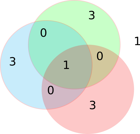
- Let R,G,B mean red, green, blue.
- P(R) = P(B) = P(G) = 1/2
- P(R and G and B) = 1/8 = P(R) P(B) P(G) so the triple is independent.
- P(R and G) = 0 != P(R) P(G) so the pair are not independent.
- You have to test every subset for independence.
- Wikipedia also talks about this.
4 Two types of testing errors
- There's an event A, with probability P[A]=p.
- There's a dependent event, perhaps a test or a transmission, B.
- You know P[B|A] and P[B|A'].
- Wikipedia:
- Terminology:
- Type I error, False negative.
- Type II error, false positive.
- Sensitivity, true positive proportion.
- Selectivity, true negative proportion.
5 Chapter 3 ctd
-
This chapter covers Discrete (finite or countably infinite) r.v.. This contrasts to continuous, to be covered later.
-
Discrete r.v.s we've seen so far:
- uniform: M events 0...M-1 with equal probs
- bernoulli: events: 0 w.p. q=(1-p) or 1 w.p. p
- binomial: # heads in n bernoulli events
- geometric: # trials until success, each trial has probability p.
-
3.1.1 Expected value of a function of a r.v.
- Z=g(X)
- E[Z] = E[g(x)] = \(\sum_k g(x_k) p_X(x_k)\)
-
Example 3.17 square law device
-
\(E[a g(X)+b h(X)+c] = a E[g(X)] + b E[h(x)] + c\)
-
Example 3.18 Square law device continued
-
Example 3.19 Multiplexor discards packets
-
Compute mean of a binomial distribution (started last Fri).
-
Compute mean of a geometric distribution (started last Fri).
-
3.3.1, page 107: Operations on means: sums, scaling, functions
-
iclicker: From a deck of cards, I draw a card, look at it, put it back and reshuffle. Then I do it again. What's the probability that exactly one of the 2 cards is a heart?
- A: 2/13
- B: 3/16
- C: 1/4
- D: 3/8
- E: 1/2
-
iclicker: From a deck of cards, I draw a card, look at it, put it back and reshuffle. I keep repeating this. What's the probability that the 2nd card is the 1st time I see hearts?
- A: 2/13
- B: 3/16
- C: 1/4
- D: 3/8
- E: 1/2
-
3.3.2 page 109 Variance of an r.v.
- That means, how wide is its distribution?
- Example: compare the performance of stocks vs bonds from year to year. The expected values (means) of the returns may not be so different. (This is debated and depends, e.g., on what period you look at). However, stocks' returns have a much larger variance than bonds.
- \(\sigma^2_X = VAR[X] = E[(X-m_X)^2] = \sum (x-m_x)^2 p_X(x)\)
- standard deviation \(\sigma_X = \sqrt{VAR[X]}\)
- \(VAR[X] = E[X^2] - m_X^2\)
- 2nd moment: \(E[X^2]\)
- also 3rd, 4th... moments, like a Taylor series for probability
- shifting the distribution: VAR[X+c] = VAR[X] (corrected from VAR[c]) [[#e4]]
- scaling: \(VAR[cX] = c^2 VAR[X]\)
-
Derive variance for Bernoulli.
-
Example 3.20 3 coin tosses
- general rule for binomial: VAR[X]=npq
- Derive it.
- Note that it sums since the events are independent.
- Note that variance/mean shrinks as n grows.
-
iclicker: The experiment is drawing a card from a deck, seeing if it's hearts, putting it back, shuffling, and repeating for a total of 100 times. The random variable is the total # of hearts seen, from 0 to 100. What's the mean of this r.v.?
- A: 1/4
- B: 25
- C: 1/2
- D: 50
- E: 1
-
iclicker: The experiment is drawing a card from a deck, seeing if it's hearts, putting it back, shuffling, and repeating for a total of 100 times. The random variable is the # of hearts seen, from 0 to 100. What's the variance of this r.v.?
- A: 3/16
- B: 1
- C: 25/4
- D: 75/4
- E: 100
-
3.4 page 111 Conditional pmf
-
Example 3.24 Residual waiting time
- X, time to xmit message, is uniform in 1...L.
- If X is over m, what's probability that remaining time is j?
- \(p_X(m+j|X>m) = \frac{P[X =m+j]}{P[X>m]} = \frac{1/L}{(L-m)/L} = 1/(L-m)\)
-
\(p_X(x) = \sum p_X(x|B_i) P[B_i]\)
-
Example 3.25 p 113 device lifetimes
- 2 classes of devices, geometric lifetimes.
- Type 1, probability \(\alpha\), parameter r. Type 2 parameter s.
- What's pmf of the total set of devices?
-
Example 3.26.
-
3.5 More important discrete r.v
-
Table 3.1: We haven't seen \(G_X(z)\) yet.
-
3.5.4 Poisson r.v.
-
The experiment is observing how many of a large number of rare events happen in, say, 1 minute.
-
E.g., how many cosmic particles hit your DRAM, how many people call to call center.
-
The individual events are independent.
-
The r.v. is the number that happen in that period.
-
There is one parameter, \(\alpha\). Often this is called \(\lambda\).
\begin{equation*} p(k) = \frac{\alpha^k}{k!}e^{-\alpha} \end{equation*} -
Mean and std dev are both \(\alpha\).
-
In the real world, events might be dependent.
-