Simulation of Simplicity (SoS) · W. Randolph Franklin

Research archive · original page Research.SoS · last recorded update 2016-03-29

Thoughts on SoS and OBLs etc.

Background of Edelsbrunner's Simulation of Simplicity (SoS)

This is a general purpose symbolic perturbation technique designed to treat special (degenerate) cases

The mathematical formalization of SoS extends the real number field of finite numbers by adding orders of infinitesimals. All positive first-order infinitesimals are smaller than the smallest positive real number. All positive second-order infinitesimals are smaller than the smallest positive first-order infinitesimal, and so on. All this is logically consistent and satisfies the axioms of a field. However, the Archimedian principle, that the ratio of any two positive elements is finite, is no longer true.

We do not actually compute with infinitesimals. Rather, we observe that their only effect is to break ties in predicates, and recode the predicates to have the effect as if they were computed with infinitesimals. This makes the code a little longer, but no slower than using only finite reals.

Basic 2D

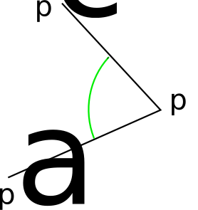
SoS worked out for the 2D angle at \(p_b\) on \(p_a p_b p_c \). I think this is correct, but could have made an error.

Without loss of generality (Wlog) let \(p_a =(0,0)\) (otherwise subtract it out.)
Notation: \( p_b=(x_b,y_b)\) etc.
\(\epsilon\) is an infinitesimal, smaller than any positive real number.
\(\epsilon^2 \lt \epsilon\) etc.
W/o SoS, the whether the angle is convex is determined by the sign of \[ D=\begin{bmatrix} x_b & y_b \\ x_c & y_c \end{bmatrix} \]

Version 1

SoS-ly translate \((x_b,y_b) \rightarrow \left(x_b+\epsilon^{2b},y_b+\epsilon^{(2b+1)}\right) \) etc.
However any choice of orders of infinitesimals would have worked; \(p_{bl} \rightarrow p_{bl}+\epsilon^{f(b,l)} \).
With SoS, the determinant \(D\) becomes \[ {\cal D} = \begin{bmatrix} x_b+\epsilon^{2b} & y_b+\epsilon^{(2b+1)} \\ x_c+\epsilon^{2c} & y_c+\epsilon^{(2c+1)} \end{bmatrix} \] \[ = \left(x_b+\epsilon^{2b}\right) \left(y_c+\epsilon^{(2c+1)}\right) - \left( y_b+\epsilon^{(2b+1)}\right)\left(x_c+\epsilon^{2c}\right) \] \[ = D + \epsilon^{2b}y_c + \epsilon^{(2c+1)} x_b - \epsilon^{2c}y_b - \epsilon^{(2b+1)} x_c \]
Define \(\text{firstsign}(a_1,a_2,a_3,...)\) to be sign of the the first argument that is nonzero, or 0.
Then compute \[\sigma=\text{firstsign}(D,y_{\max(b,c)},-x_{\max(b,c)},-y_{\min(b,c)},x_{\min(b,c)})\]
\(\sigma=0\) only when all the points are 0.
The answer depends on how the points are ordered. Since breaking ties is breaking a symmetry, something has to be nonsymmetric in the rule. We shouldn't care how we break the ties (degeneracies), so long as we do it consistently throughout the whole problem.
Nevertheless, this should consistently label angles in a planar mesh.
If \(p_{\max(b,c)}\ne o\) then if \(y_{\max(b,c)}=0\) then \(x_{\max(b,c)}\ne0\)
Then this can be simplified to \[\label{eqn1} \sigma=\text{firstsign}(D,y_{\max(b,c)},-x_{\max(b,c)}) \]

Version 2

Simplify the above even more, by letting the id of \(p\) be its order when all the \(p\) are sorted lexicographically.
Let \(i\) be \(b\) or \(c\) depending on whether \(y_b\) or \(y_c\) is larger.
Let \[i=\left\{\begin{matrix} \text{if } y_b>y_c \vee (y_b=y_c\wedge x_b>x_c) & \text{ then } & b\\ &\text{ else }& c \end{matrix} \right. \]
Then Equation (1) above becomes \[\sigma=\text{firstsign}(D,y_i,-x_i)\]

3D

Consider two triangles, \(\bigtriangleup o p_a p_b\) and \(\bigtriangleup o p_a p_c\) with a common edge \(o p_a\).
\( a, b, c \) are the integer indices of the points in the points array. \( 0\le a, b, c \lt n \).
We want the answer to the question, is the dihedral angle on that edge convex?
This depends on the sign of the determinant \[ D = \begin{bmatrix} p_a & p_b & p_c \end{bmatrix} = \varepsilon_{ijk}\, p_{ai}\,p_{bj}\,p_{ck} \]
That used the Einstein tensor notation:
\( \varepsilon_{ijk} = -1, 0, \text{or } 1\), depending on whether \(ijk\) is a positive permutation, have an index duplicated, or is a negative permutation.
sum over doubled indices.
SoS transform \( p_{ai} \rightarrow p_{ai} + \epsilon^{a+ni} \) (other choices are possible).
\[ {\cal D} = \varepsilon_{ijk}\, (p_{ai}+\epsilon^{a+ni})\, (p_{bj}+\epsilon^{b+nj})\, (p_{ck}+\epsilon^{c+nk}) \] \[ = D + \\ \varepsilon_{ijk} \left( \epsilon^{a+ni} p_{bj} p_{ck} + \epsilon^{b+nj} p_{ai} p_{ck} + \epsilon^{c+nk} p_{ai} p_{bj} \right) + \\ \varepsilon_{ijk} \left( \epsilon^{b+c+n(j+k)} p_{ai} + \epsilon^{a+c+n(i+k)} p_{bj} + \epsilon^{a+b+n(i+j)} p_{ck} \right) + \\ \varepsilon_{ijk} \left( \epsilon^{a+b+c+n(i+j+k)} \right) \] \[ = D + \\ \epsilon^a (p_{b1} p_{c2} - p_{b2} p_{c1}) + \epsilon^b (p_{a1} p_{c2} - p_{a2} p_{c1}) + \epsilon^c (p_{b1} p_{a2} - p_{b2} p_{a1}) + \text{ higher order terms} \]
Let \(a'=\min(a,b,c),\ b'=\text{median}(a,b,c),\ c'=\max(a,b,c)\). Then, apart from possible sign errors, the angle is convex depending on \[ \sigma = \text{firstsign}(D, (p_b' \times p_c')_2, (p_c' \times p_a')_2, (p_a' \times p_b')_2) \]
This fails when the vectors are collinear. The omitted higher order terms could handle them.
Still do to: Include ordering points by coordinates, as above for 2D.

2 Intersecting lines

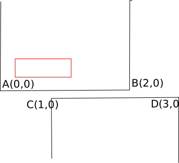
Perturb
\(B(2,0)\rightarrow (2+\epsilon, \epsilon^2)\)
\(C(1,0)\rightarrow (1+\epsilon^3, \epsilon^4)\)
\(D(2,0)\rightarrow (3+\epsilon^5, \epsilon^6)\)
The slope of the line through A(0,0) and \(B(2+\epsilon, \epsilon^2)\) is \[ \frac{\epsilon^2}{2+\epsilon} \]
This could probably be simplified to \[ \frac{\epsilon^2}{2} \] The hi order terms would be relevant only if the lo order terms later cancelled.
AB's equation is \[ y = \frac{\epsilon^2}{2+\epsilon} x \] possibly simplified to \[ y = \frac{\epsilon^2}{2} x \]
The slope of the line through \(C(1+\epsilon^3, \epsilon^4)\) and \(D(3+\epsilon^5, \epsilon^6)\) is \[ \frac{\epsilon^6-\epsilon^4}{3+\epsilon^5-1-\epsilon^3} \]
CD's equation is \[ y = \frac{\epsilon^6-\epsilon^4}{2+\epsilon^5-\epsilon^3} x + \frac{3\epsilon^4-\epsilon^6}{2+\epsilon^5-\epsilon^3} \]
It could probably be simplified to \[ y = -\frac{\epsilon^4}{2} x + \frac{3\epsilon^4}{2} \]
Then, using the simplified expressions, AB and CD intersect at \[ \left(-3\epsilon^2,-\frac{3}{2}\epsilon^4\right) \]
Since AB's positive slope is greater than CD's negative slope, A and B are above CD, while C and D are below AB. So the above figure is correct.
Now consider this figure:

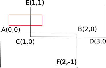
Since AB is above CD here, edges AB and CE should intersect.
So, in this case, things work out.

B-rep

What does SoS do to the intersection of two coincident lines? Might the intersection after the perturbation be far away?

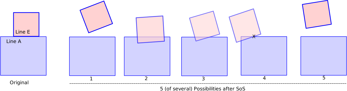
Let lines A and E be \(y=0\).
After SoS, A becomes \(y=\epsilon^4 x + \epsilon^8\) and E becomes \(y=\epsilon x + \epsilon^2\). E has a slightly greater slope than A.
(If my math is right) they intersect at \[ (x,y) = \left( -\epsilon\ \frac{1-\epsilon^6}{1-\epsilon^3}, \ -\epsilon^5\right) \]
Approximately, \[ (x,y) = (-\epsilon, \ \epsilon^5) \] so case 5 above obtains.
How might we make the intersection to be far away?
Two general lines are \(y=ax+b\) and \(y=cx+d\).
They intersect at \[(x,y) = \left( \frac{d-b}{a-c},\ \frac{ad-bc}{a-c} \right) \]
Since the lines are coincident, let \(c=a\) and \(d=b\).
SoS-ify to make the lines \[y=(a+\epsilon)x+(b+\epsilon^2)\] and \[y=(a+\epsilon^4)x+(b+\epsilon^8)\]

They will intersect at \[(x,y) = \left( \frac{b+\epsilon^8-b-\epsilon^2}{a+\epsilon-a-\epsilon^3}, \ \frac{ \epsilon b-\epsilon^2 a -\epsilon^4 b-\epsilon^6+\epsilon^8a+\epsilon^9}{a+\epsilon-a-\epsilon^3} \right) \] \[ = \left(-\epsilon\frac{1-\epsilon^6}{1-\epsilon^2},\ \frac{ b-\epsilon a-\epsilon^3 b-\epsilon^5+\epsilon^7 a+\epsilon^8}{1-\epsilon^2} \right) \] ignoring higher order terms \[ = \left(-\epsilon,\ b-\epsilon a-\epsilon^5 \right) \]
Conclusion: the intersection point is never way off in the distance.

B-rep and concavity

Will SoS cause the perturbed polygon to have a concavity at the new intersection?

See case 4 in the above figure, with the intersection at X.
To make X to be on the edge (and not on its extension), \(\epsilon\) will have to be negative. Ok.
W/o doing the math, I'm guessing that concavities can occur, with the resulting in a polygon having a spike.

Indeed, if the intersection was convex on 1 side then it would have to be concave on the other.
Regularization would be needed to fix this.
However, it is possible that if I worked out the details, something nice would actually happen.

Thoughts on Optimized Boolean Lists

Stencil buffers have been deprecated since OpenGL 3.0 in 2008. However OpenGL 3.0 has taken years to catch on, because of various flaws.
GPUs are now general enough that you can implement stencil buffers yourself.
An efficient design would depend on the number and complexity of the primitives.
Also, data movement is often more expensive than computation.
Therefore, I propose implementing the following version 1 first.
Store the primitives' definitions in the GPU, perhaps procedurally, would seem best.
That is, in CUDA terms, have a device function for each primitive, which takes a pixel location and returns 0 or 1. Name it, the primitive's characteristic function.
Use a CUDA thread for each pixel, which calls each primitive's characteristic function on that pixel, and evaluates the Boolean expression.
Another idea would be to use a thread for each (pixel, primitive) pair. Since that requires more threads than CUDA cores, it would seem to be slower, unless the threads running different functions used different limited resources simultaneously, and so could be scheduled better.
The above design would be suboptimal if calling a primitive's characteristic function separately for each pixel is much slower than computing the primitive's stencil all at once, even when including the cost of storing and later accessing the stencil.
Nothing in the above notes is restricted to 2D because current GPU hardware doesn't care. For several years, the highest performance GPUs have not even had video out.
My 3-year-old GPU, an Nvidia K20xm, has 6GB of global memory (although not all usable). Allocating one byte for each of \(1024^3\) voxels is quite feasible; one bit each, even more so.
Using one byte/voxel would allow labeling a voxel with, e.g., color.
I.e. now, one billion is not a large number.
However, is that enough for hi quality manufacturing?
The slowest part might well be writing to that common global array, since global memory is slow. However, because successive threads write to successive bytes, it might well be fast. We'd have to try it and see.
Coding in Thrust, the functional API on top of CUDA, would be easier. One advantage is that you can develop the code w/o having CUDA, and then just change the backend.
If version 1 is implemented, and measurements confirm that it is too slow, then we can consider optimizations like these.
Recoding in CUDA.
Partitioning the output array into pieces each small enough to store in a fast cache, and combining the pieces later.
If there were many small primitives, then bucket sorting them with a uniform grid would allow a pixel to evaluate only those primitives likely to overlap it.
It's difficult to make more specific suggestions w/o knowing more specifics about the application.
I could write a prototype of version 1 if you're interested. What type (analytic spheres, cubes, ...), size, and number of primitives would be interesting?
Still to think about: the really cool trimming and active zone techniques mentioned in the talk.

Continuing the intersection of two edges

Given two edges AB and CD, with A(0,0), B(2,0), C(1,0) and D(3,0).
Perturb
\(B(2,0)\rightarrow (2\pm\epsilon^a, \pm\epsilon^b)\)
\(C(1,0)\rightarrow (1\pm\epsilon^c, \pm\epsilon^d)\)
\(D(2,0)\rightarrow (3\pm\epsilon^e, \pm\epsilon^f)\)
Use \(a,b,c,d,e,f\) to control how SoS operates.
That's not fully general since I'm not perturbing A (for now).
The slope of AB is \[\frac{\pm\epsilon^b}{2\pm\epsilon^a} \]
The slope of CD is \[\frac{\pm\epsilon^f\mp\epsilon^d}{2\pm\epsilon^e\mp\epsilon^c} \]
AB's equation is \[ y=\frac{\pm\epsilon^b}{2\pm\epsilon^a} x \]
CD's equation is \[ y=\frac{\pm\epsilon^f\mp\epsilon^d}{2\pm\epsilon^e\mp\epsilon^c}(x\mp\epsilon^c)\pm\epsilon^d \]