Research archive · original page Research.June2006AnnualReport · last recorded update 2006-10-28
DARPA/DSO/GEO*: Geologically Correct Terrain Data Structures and Radar Siting, Annual Report, June 2006
Professional Personnel
Various personnel, ranging from faculty members to grad students and undergrad students, are currently being supported by the project.
- Dr W. Randolph Franklin, Associate Professor, RPI, `PhD (Applied Math, Harvard): Strategizing, managing, writing, prototype coding, (parttime on this project during the academic year, two months in summer).
- Dr Caroline Westort, Research Assistant Professor, RPI, `PhD (Geography, Zürich): Strategizing about scooping, (fulltime from August 2005).
- Dr Frank Luk, Professor, RPI, `PhD (Computer Science, Cornell): Numerical analysis advice, (two months this summer). Prof Luk is a former chair of CS, and is an internationally renowned expert in Scientific Computation.
- Metin Inanc, Research Assistant and `PhD candidate (RPI): Incremental TIN, using ODETLAP to fill in missing data holes, the scooping alternative terrain representation, (halftime during the academic year, fulltime in the summer).
- Zhongyi Xie, Research Assistant and `PhD candidate (RPI): Using ODETLAP to reconstruct a surface from the minimal number of points generated by a TIN, (halftime during the academic year, fulltime in the summer).
- Dan Tracy: `PhD candidate (RPI): SVD approximations, multiobserver siting, path planning, (supported as a Teaching Assistant during Spring 2006, supported as a Research Assistant on the contract halftime during the academic year starting Fall 2006, fulltime in the summer starting 2006).
- Jared Scheuer, junior: studied aspects of ODETLAP during summer 2005. He measured the accuracy of either subsampling the surface, or of having a region of missing data, and using this technique to fill in the missing data.
- Rositsa Tancheva, junior: researched non photorealistic rendering (NPR) in computer graphics, in order to apply that to terrain. This was exploratory work that might lead to another new representation.
- John Shermerhorn, junior: also looking at some terrain issues, such as creating a testbed in which we can try our ideas.
- Joe Roubal, ESRI: implementing the multiobserver siting toolkit in `ArcGIS.
- Steve Martin, undergrad (RPI): working during summer 2006 on sculpting terrain for Prof Westort.
- COL Clark Ray, `PhD, provided valuable advice while at the USMA West Point. However, he has since retired from the Army, and unfortunately is no longer active on this project.
Project Goals
These may be summarized as follows.
- Study alternate terrain representations that are more compact.
- Since the new representations will therefore be lossy, evaluate the size / quality tradeoffs.
- These new representations ought to make it easier to represent legal terrain than illegal terrain.
- We wish to process datasets up to 10000x10000 elevation posts.
- With these new representations, uncompression speed is more important than compression speed.
- The new representations are to be evaluated on metrics such as visibility and mobility.
Summary of Accomplishments and Status
We are proceeding with researching alternative, more compact, representations of elevation data. We are now combining the various representations for greater power. Our initial evaluations of our alternative representations use, in addition to RMS elevation error, the observer siting and visibility metric. We are starting to employ the mobility metric. Here are some sample results.
- Our incremental Triangulated Irregular Network (TIN) program can process a 10800x10800 array of posts in internal memory on a PC. The accuracy is impressive; one dataset uses only 157,735 triangles to represent the 11,664,000 posts to a 3% maximum elevation error.
- Our scooping representation processed the `W111N31 cell with 7x7 linear scoops to an average elevation error of 0.1%, and maximum error of 2%.
- We represented one 3592x3592 dataset with 7x7 scoops, and then compared the joint viewsheds resulting from multiobserver siting on the original representation and the alternate. The error was only 6.5%.
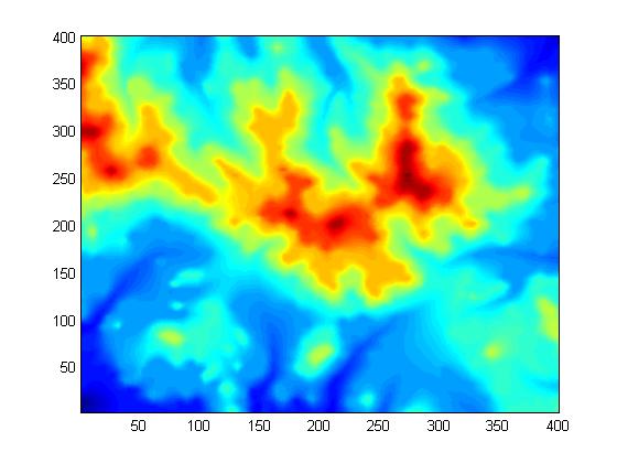
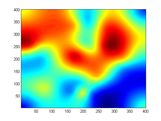
- We tested another new representation, ODETLAP, on a 400x400 piece of the Lake Champlain W cell. After selecting every third post in each of X and Y, that is 1/9 of the points, and using ODETLAP to fit a surface to them, the error was only 0.9 meters, or 0.1% of the elevation range.
- We are combining TIN with ODETLAP, in order to capture the essence of a surface with very few points.
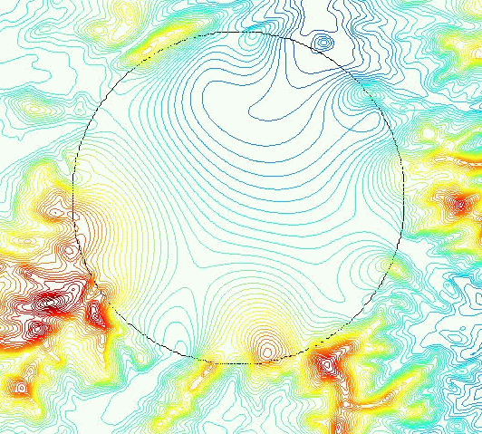
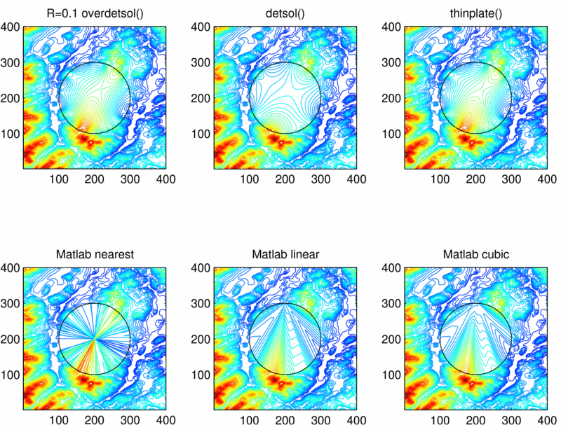
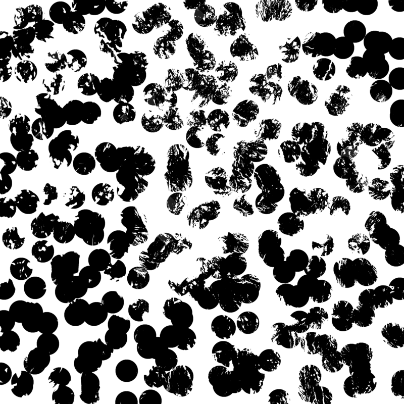
- We can use ODETLAP to fill in radius 40 circles of missing data, with excellent results.
Test Datasets and Protocols
These experiments used the following test datasets:
- USGS Lake Champlain W 1° DEM, which has a good mix of mountains, including Mt Marcy (the NYS highpoint), lowlands, and Lake Champlain.
- DTED level 2 data from the March 2005 kickoff meeting.
- SRTM DTED level 2 data from `CDs supplied in January 2006.
Of that data, we're standardizing on these mountainous cells: w119n36.dt2, w120n38.dt2, w121n45.dt2, w112n41.dt2, w112n40.dt2. Per an NGA request in February 2006, we added some less mountainous cells: w112n32.dt2, w113n32.dt2, w113n33.dt2, w113n40.dt2, w113n41.dt2, w114n32.dt2, w114n33.dt2, w115n33.dt2, w119n33.dt2.
Our several testing protocols operate as follows.
- Compute some property on the original terrain representation, which is a large matrix of elevation posts
- Compute that property again on the alternative representation, whether TIN, scooping, or ODETLAP.
- Measure the difference between the two representations.
- Evaluate various test datasets.
- Examine the tradeoff between the size of the dataset and its quality.
Some of the various test protocols are the following.
- Protocol 1: Elevation Testing. Here we measure both average absolute error and RMS error. The reason is that some representations do better at one than at the other. In addition, we examine the terrain to see if its features are captured. This is important but hard to quantify.
-
Protocols 2-4: Visibility Testing. These contain various
levels of complexity:
- Evaluate differences in observer viewsheds.
- Evaluate the visibility index of every observer in the cell.
- Evaluate multiobserver siting quality.
-
Protocol 2: Viewshed Testing, which proceeds as follows.
- Select values for the following parameters: Radius of interest, R, and observer and target heights, H.
- Compute the viewshed bitmaps of many observers on both the original and the alternative representations. We can do this fast even for large R.
- For some observer O, let V'_o_' be its viewshed on the original, and V'_a_' be its viewshed computed on the alternative representation. V'_o_' and V'_a_' are bitmaps (i.e., sets of target points visible by O). Report the size of the symmetric difference, |V'_o_'-V'_a_'| + |V'_a_'-V'_o_'|.
-
Protocol 3: Visibility Index Testing:
- Consider each post in term as an observer.
- Compute its visibility index.
- Using Monte Carlo sampling, pick T random targets, compute their visibility, and report the fraction visible.
- Produce a map of all the visibility indexes.
- Compare the visibility index map of the original terrain representation to the map of the alternative representation.
-
Protocol 4: Multiple Observer Siting Testing
- Site a set of observers, S'_o_', on the original terrain representation.
- Site a set of observers, S'_a_', on the alternative terrain representation.
- Transfer S'_a_' to the original representation.
- Compare the quality of S'_a_' to that of S'_o_'.
Alternative Terrain Representations
Our alternative terrain representations are as follows.
- TIN
- Scooping
- ODETLAP
- Combinations of the above, e.g., ODETLAP uses TIN points.
It is important to note that good compression techniques are multistep. For instance, JPEG combines the following sequential steps:
- Rotate from the RGB colorspace to the `YCrCb colorspace.
- Perform a discrete cosine transform.
- Perform a low-pass filter.
- Arithmetic encode the remaining coefficients.
Text compression, e.g. bzip2, performs the following steps in sequence.
- Run length encoding.
- Burrows-Wheeler transformation.
- Move to front.
- Another run length encoding.
- Arithmetic encoding.
Our ultimate recommendation may well be a combination of our various techniques, perhaps as follows:
- Reconstruct an approximate surface with scooping, or
- Select significant points with TIN.
- Smooth the surface with ODETLAP.
- Fill in any local minima with our fast connected component program. (This program designed to process 3D cubes of bits, up to 600x600x600 voxels, resulting from threshholding a CAT scan. However, it can process 2D datasets as a special case. For example, one 18573x19110 image took 25 CPU seconds to process on a 1600 MHz laptop.)
Note that the last two steps do not increase the information content of our representation. That is, if they are a fixed part of our reconstruction engine, having them operate adds zero bits to the representation of the terrain.
Some experiments were performed by Tracy to compress the terrain using the singular value decomposition (SVD.) Various methods of partitioning the terrain and performing an SVD on each partition were tested. The results were inferior to those of competing compression methods. However, the SVD may still be useful in combination with other compression methods, such as scooping.
TIN
Features
Our version is a progressive resolution method.
- The initial TIN is just two triangles partitioning the cell.
- At each step, the post whose elevation is vertically farthest from the triangle containing its projection onto the XY plane is inserted into the triangulation, splitting one triangle into three.
- Often that point lies on an edge of the triangulation. In that case, one triangle is degenerate.
- If the new point lies on the cell's border, then its triangle is split into only two triangles.
- If necessary, a few edges are flipped to maintain the triangulation as Delauney. If one of the new triangles is degenerate, then one of its edges will always be flipped, removing the degeneracy.
This progressive resolution property is not common to some other triangulation methods, which may process the whole set of points at once. Our method may be stopped when any precondition is met. Typical preconditions include the insertion of a predetermined number of points, or the attainment of a predetermined maximum absolute error.
The points that have been inserted at that time are, in some sense, the most important points in the surface. They may then be used by a successive process such as ODETLAP. Since this point may not be widely appreciated, Figure 1 shows an example constructed to be difficult. The test dataset contains two overlapping circular ridges with sharp tops, transected by a railroad embankment with vertical sides.
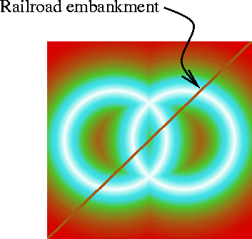
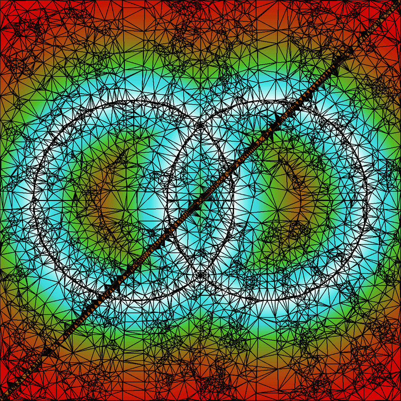
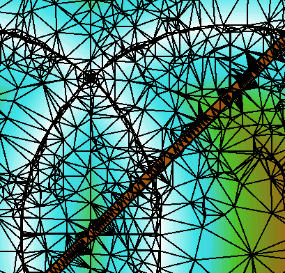
Figure 2 shows the result of applying TIN until the maximum error is sufficiently small. Note how points are selected along the ridges and embankment sides, and how the edges align with these features and do not cross them. Figure 3 is an enlarged detail.
The data structures used by our TIN method were the result of considerable thought before the first line of code was written. They are very compact, which is why we can process such large cells on a PC. For example, edges are not stored explicitly, but rather, each triangle has pointers to its (one to three) neighboring triangles. That saves space, at the cost of slowing down edge flips.
Feature points on the peaks and ridgelines, and the edges joining them, may be more important properties of the surface. Our TIN program selects them automatically; there is no need for manual identification and constrained triangulation. The points selected for the triangulation are assumed to be important, and can be fed into other methods, like ODETLAP. TIN is a piecewise linear triangular spline. Preliminary experiments with a higher degree spline showed no consistent improvement, and so were suspended.
Improvements This Year
Inanc modularized the TIN program and changed it in several ways. The error handling was changed to use C++'s exception handling mechanism. The code in the main() was removed and a new function was created to include the meta tasks for tinning. The Boost library's arrays were used for output.
Preliminary Testbed
A testbed using Python and the windowing library `WXWin, (`WXWidgets) was attempted. It was observed that the `WXWin bindings (`WXWin is a C++ library) for Python are not very stable. A side product was a GUI for the tinning program. The experimental testbed has a sluggish UI which is connected to a couple of C++ modules used to tin DEMs, render DEM files and render resulting TINs. A new testbed implementation is being built using Java, backed up by Matlab. This is justified by the fact that Java classes can be used natively within Matlab (Matlab's own GUI is Java based) and Java provides a rich set of libraries for building GUI and for scientific tasks. The new testbed is scooping/segmentation oriented.
Status
We can process 10800x10800 arrays of posts in 1/2 hour on a PC. No external storage is used. Our test dataset was formed by catenating nine 3601x3601 cells of data from the Savannah March kickoff meeting.
The elevation range of the dataset is 3600. `TINning it until the maximum absolute error was 100, i.e., 3%, produced 157,735 triangles in 1292 CPU seconds. `TINning it until the maximum absolute error was 10, i.e., 0.3%, produced 5.320,089 triangles in 1638 CPU seconds.
Lossless TIN
TIN is inherently lossy, but we can make it lossless as follows.
- Fit a surface to the TIN points, using any method.
- Compute the errors.
- Compress tue errors, say with `PAQ3N.
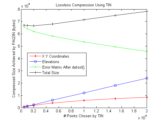
The more TIN points that are used, the more accurate the reconstructed lossy surface will be, and the less space will be needed to code the errors. The goal is to minimize the sum of the two sizes. Figure 4 shows the tradeoff when using the Laplacian PDE to interpolate the points. Other methods, such as ODETLAP, would be better.
The {(x,y,z)} TIN points must finally be coded. In this, note that the order of the set elements is immaterial. Bitmap coding techniques suffice for {(x,y)}. Assuming that there is not structure and that the points are random, there is an information theoretic limit. The coding of the (x,y) now determines the order of the zs. They may be compressed with a sequence of Burrow Wheeler, run length and arithmetic coding.
Scooping
This representation is longterm research. The goal is to smash through the information theoretic barrier to terrain compression by utilizing geologic information. We are pursuing several representations in parallel.
Several different shaped scoops were tried by Inanc. The most primitive scoops are flat-bottom scoops (0-degree equations). They are very effective in representing areas like seas, oceans, lakes, plateaus and any naturally occuring flat areas. In contrast, a Morse description is totally at loss with those structures. Our initial efforts concentrated on working with square shaped drills. The problem with those is that natural terrain does not segment easily into squares. Thus to represent a lake many square shaped scoops are required. An improvement was developing hierarchical scooping akin quad-tree representation. Thus if a single square is too big it will result in a representation error beyond a threshold and thus will be subdivided internally into smaller squares. To decrease the number of scoops more elaborate models were tried. 1-degree scoops are still flat, however a full blown planes which can be tilted to represent slopes. 2-degree scoops use quadratic equations and are still more versatile. 3-degree scoops (cubics) use prohibitively many parameters (10 coefficients). However with the increase of the degree of scoops the number of scoop applications required to represent the terrain accurately decreases.
A next and natural step is to build a segmentation algorithm which can take care of the natural shapes of geological formations. A constructive algorithm for segmentation can start by growing segments around seeds of initially selected points. If a point coincides with a lake the segment can be expected to grow to the full lake size merging other segments thus representing the whole lake with a single 0-degree flat-bottom scoop. The problem here is representing shapes. There are different ways to represent 2D shapes. The simplest way is to use bitmaps. Those can be compressed using fax compression algorithms. More complicated methods use Voronoi diagrams and build a skeleton to represent shape.
Some of the tests will now be described in more detail.
Degree-0 Scoops
The purpose of this was to learn what types of drills are more useful by implementing a Matlab test program. It is a greedy optimization - at each step, select the drill instance and location
(drill type, x, y, z)
that removes the most material. Drill instances will generally overlap. If two drills drill the same post, then the minimum elevation is used. This nonlinearity is radically different from, and more powerful than, wavelets. This nonlinearity also matches physical reality. If a river valley that cut 200' below the surrounding plane meets another river that is cut only 100' deep, then, at the confluence, the valley is only 200' deep, not 300'.
There are various subtleties of the greedy optimization. The drill that removes the most material at the start may be rendered completely redundant by later drills. This is reminiscent of stepwise multiple linear regression, where an initially important variable may ultimately be unimportant. A future possibility is to remove as well as add drills to the set. However this would be more compute intensive.
After the drills are determined, the final step would be encoding them. Note that the order of the drill applications is immaterial. Therefore, when coding, all the instances of the same drill may be grouped together. Then it is possible to sort the instances by location and delta encode the locations, since successive instances are relatively close. Alternatively a good bitmap compression method, such as CCITT group 4, could be used to code the drill locations.
The initial drills had no parameters other than their (x,y) location and (z) depth. One generalization, discussed in more detail later, is to allow more general (sloped) drills. This would tradeoff powerful, large to encode, basis elements, against small simple elements. However more of the simple more would be needed than of the complex ones. The sweet point would probably occur when the basis elements resemble the object being approximated. The purpose of these experiments is to better understand scooping, while initiating experiments in slope-preservation during lossy compression. The underlying assumption is that there is little long range correlation of elevation or slope.
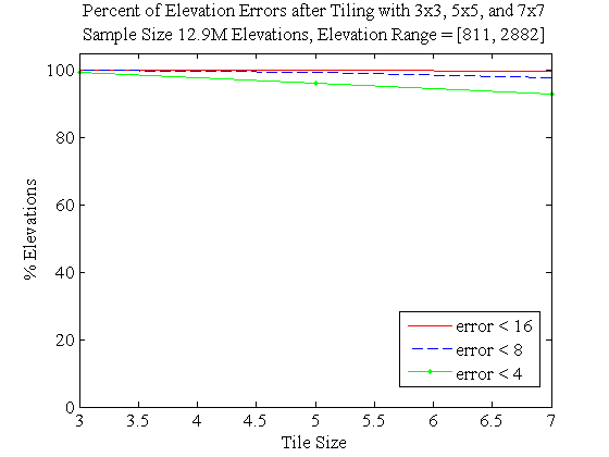
An initial test on the 1201x1201 Lake Champlain West cell had these results. There were 11 drill types: a square of size 1 or 3, a circle of diameter 5, 10, or 20, a parabola of size 5, 10, or 20, and a flatter parabola of size 5, 10, or 20. After 10,000 drill instances, the initial material volume of 1.9x10'^9^' was reduced to 4.2x10'^7^'. The mean absolute elevation among the 1201'^2^' posts was 30m, or 2% of the elevation range. 98% of the selected drill instances were the diameter 20 circle, with the diameter 10 circle and size 3 square distantly behind. The parabola drills were not selected even once. Table 1 gives the complete results.
| border=1 | ||||||
| id=drillfreq | ||||||
| !Drill Type | !Count | |||||
| Square, D=1 | 0 | |||||
| Square, D=3 | 35 | |||||
| Circle, D=5 | 2 | |||||
| Circle, D=10 | 129 | |||||
| Circle, D=20 | 9834 | |||||
| Parabola, size 5 | 0 | |||||
| Parabola, size 10 | 0 | |||||
| Parabola, size 20 | 0 | |||||
| Flatter parabola, size 5 | 0 | |||||
| Flatter parabola, size 10 | 0 | |||||
| Flatter parabola, size 20 | 0 | |||||
| ! Representation | ! % Error | |||||
| tile3 | 1.31% | |||||
| tile5 | 3.67% | |||||
| tile7 | 6.52% | |||||
| tile75 | 5.62% | |||||
| !K | !Data set size, % | !Error | !Error % | |||
| 3 | 11.1% | 0.9 | 0.065% | |||
| 4 | 6.25% | 1.6 | 0.11% | |||
| 5 | 4% | 2.4 | 0.17% | |||
| 7 | 2% | 4.1 | 0.29% | |||
| 10 | 1% | 6.5 | 0.46% | |||
| 15 | 0.44% | 10 | 0.71% | |||
| 20 | 0.25% | 12 | 0.86% | |||
| 30 | 0.11% | 14 | 1.0% | |||
| 50 | 0.05% | 16 | 1.1% | |||
| !Abbrev | !Meaning | |||||
| TIN a | TIN, average error | |||||
| Reg a | Regular, average error | |||||
| Ref a | Refined TIN, average error | |||||
| TIN m | TIN, max error | |||||
| Reg m | Regular, max error | |||||
| Ref m | Refined TIN, max error | |||||
| !Data | !Reg a | !TIN a | !Ref a | !Reg m | !TIN m | !Ref m |
| `W111N3110 | 3.4 | 5.6 | 5.3 | 98 | 31 | 27 |
| `W111N3111 | 9.0 | 10.6 | 10.4 | 134 | 113 | 66 |
| `W111N3112 | 1.7 | 2.7 | 2.6 | 114 | 20 | 16 |



Notes
- John Childs masters, A Two-Level Iterative Computational Method for Solution of the Franklin Approximation Algorithm for the Interpolation of Large Contour Line Data Sets, http://www.terrainmap.com/
- http://www.ecse.rpi.edu/Homepages/wrf/Research/geostar-reports/fill_data_holes/index.html
- http://www.ecse.rpi.edu/Homepages/wrf/pmwiki/GeoStar/