Engineering Probability Final Exam Notes Wed 2021-05-12

1 Status, Wed 2021-05-12

  1. Day 6 of the outage.

  2. ECSE-2500 Engineering Probability grade modification because the optional final was canceled: Replace the final grade with the max of the other 2 exams, then use the top 2 of the 3 exams. Then add 5% to everyone's total grade. This makes the course GPA 3.36, which ain't so bad.

  3. I can't access SIS yet to upload the grades to the registrar. However I will try to upload them to LMS FYI.

2 Status, Mon 2021-05-10

  1. Day 4, hackers have taken RPI off the internet, and I don't know when it will be back up. Higher levels at RPI are silent about what happened, and when RPI will be back online.

  2. The final exam has been canceled. There will not be a makeup. This is RPI policy. It is also the only reasonable thing to do.

  3. RPI levels above my pay grade will decide a grading policy. We would like some consistency between courses.

  4. This site, https://wrandolphfranklin.org/probability , will have updates. Although it's now moot, it also has a copy of my course blog, with links updated.

  5. If you send me your non-RPI email, I'll email announcements. You may email me at PEE ARR OH BEE AT DOUBLEYOU ARR EFF ARR EH EN KAY ELL EYE EN DOT OH ARR GEE, and also ask questions.

  6. ECSE's new temporary website has ECSE updates and a form to enter your contact info.

3 More online material

  1. The lecture videos . (I keep local copies of most everything.)

  2. Last year's final exam. Answers .

Engineering Probability Class 26 and Final Exam Mon 2020-04-27

Table of contents::

1 Rules

  1. You may use any books, notes, and internet sites.

  2. You may use calculators and SW like Matlab or Mathematica.

  3. You may not ask anyone for help.

  4. You may not communicate with anyone else about the course or the exam.

  5. You may not accept help from other people. E.g., if someone offers to give you help w/o your asking, you may not accept.

  6. You have 24 hours.

  7. That is, your answers must be in gradescope by 4pm (1600) EDT Tues.

  8. Email me with any questions. Do not wait until just before the due time.

  9. Write your answers on blank sheets of paper and scan them, or use a notepad or app to write them directly into a file. Upload it to gradescope.

  10. You may mark any 10 points as FREE and get the points.

  11. Print your name and rcsid at the top.

2 Questions

  1. Consider this pdf:

    $f_{X,Y} (x,y) = c (x^2 + 2 x y + y ^2) $ for $ 0\le x,y \le 1 $, 0 otherwise.

    1. (5 points) What must $c$ be?

    2. (5) What is F(x,y)?

    3. (5) What is the marginal $f_X(x)$?

    4. (5) What is the marginal $f_Y(y)$?

    5. (5) Are X and Y independent? Justify your answer.

    6. (30) What are $E[X], E[X^2], VAR[X], E[Y], E[Y^2], VAR[Y]$ ?

    7. (15) What are $E[XY], COV[X,Y], \rho_{X,Y}$ ?

  2. (5) This question is about how late a student can sleep in before class. He can take a free bus, if he gets up in time. Otherwise, he must take a $10 Uber.

    The bus arrival time is not predictable but is uniform in [9:00, 9:20]. What's the latest time that the student can arrive at the bus stop and have his expected cost be no more than $5?

  3. (5) X is a random variable (r.v.) that is U[0,1], i.e., uniform [0,1]. Y is a r.v. that is U[0,X]. What is $f_Y(y)$ ?

  4. (5) X is an r.v. U[0,y] but we don't know y. We observe one sample $x_1$. What is maximum likelihood for y?

  5. This is a noisy transmission question. X is the transmitted signal. It is 0 or 1. P[X=0] = 2/3. N is the noise. It is Gaussian with mean 0 and sigma 1.

    Y = X + N

    1. (5) Compute P[X=0|Y].

    2. (5) Compute $g_{MAP}(Y)$.

  6. Let X be a Gaussian r.v. with mean 5 and sigma 10. Let Y be an independent exponential r.v. with lambda 3. Let Z be an independent continuous uniform r.v. in the interval [-1,1].

    1. (5) Compute E[X+Y+Z].

    2. (5) Compute VAR[X+Y+Z].

  7. (5) We have a Gaussian r.v. with unknown mean $\mu$ and known $\sigma = 100$. We take a sample of 100 observations. The mean of that sample is 100. Compute $a$ such that with probability .68, $100-a \le \mu \le 100+a$.

  8. (5) You're testing whether a new drug works. You will give 100 sick patients the drug and another 100 a placebo. The random variable X will be the number of days until their temperature drops to normal. You don't know in advance what $\sigma_X$ is. The question is whether E[X] over the patients with the drug is significantly different from E[X] over the patients with the placebo.

    What's the best statistical test to use?

  9. You're tossing 1000 paper airplanes off the roof of the JEC onto the field, trying to hit a 1m square target. The airplanes are independent. The probability of any particular airplane hitting the target is 0.1%. The random variable X is the number of airplanes hitting the target.

    1. (5) What's the best probability distribution for X?

    2. (5) Name another distribution that would work if you computed with very large numbers.

    3. (5) Name another distribution that does not work in this case, but would work if the probability of any particular airplane hitting the target is 10%

      Historical note: for many years, GM week had an egg toss. Students designed a protective packaging for an egg and tossed it off the JEC onto the brick patio. Points were given for the egg surviving and landing near the target.

    4. You want to test a suspect die by tossing it 100 times. The number of times that each face from 1 to 6 shows is this: 12, 20, 15, 18, 15, 20.

      1. (5) What's the appropriate distribution?

      2. (5) If the die is fair, what's the probability that the observed distribution could be that far from the actual probability?

Total: 140 points.

Engineering Probability Class 26 Mon 2021-05-03

1 Grade

  1. There will be no homework assigned today. Homework 21, due today, was the last.

  2. Per the syllabus, the lowest of your 3 exam grades will be dropped.

  3. In a day or so, I will calculate your guaranteed grade if you don't write the final, and try to post it on LMS.

  4. If you write the final, it can only raise your grade.

  5. In a few days, I might post a survey to see if anyone at all wants to write the final.

  6. In particular if you're in China and want to write the final 12 hours later, then write me. Only people now physically in east Asia or similar places are allowed to do this.

2 No video for class 25

Something didn't work.

(The 25 is a correction; earlier I said 24.)

3 Review questions

  1. What is $$\int_{-\infty}^\infty e^{\big(-\frac{x^2}{2}\big)} dx$$?

    1. 1/2

    2. 1

    3. $2\pi$

    4. $\sqrt{2\pi}$

    5. $1/\sqrt{2\pi}$

  2. What is the largest possible value for a correlation coefficient?

    1. 1/2

    2. 1

    3. $2\pi$

    4. $\sqrt{2\pi}$

    5. $1/\sqrt{2\pi}$

  3. The most reasonable probability distribution for the number of defects on an integrated circuit caused by dust particles, cosmic rays, etc, is

    1. Exponential

    2. Poisson

    3. Normal

    4. Uniform

    5. Binomial

  4. The most reasonable probability distribution for the time until the next request hits your web server is:

    1. Exponential

    2. Poisson

    3. Normal

    4. Uniform

    5. Binomial

  5. If you add two independent normal random variables, each with variance 10, what is the variance of the sum?

    1. 1

    2. $\sqrt2$

    3. 10

    4. $10\sqrt2$

    5. 20

  6. X and Y are two uniform r.v. on the interval [0,1]. X and Y are independent. Z=X+Y. What is E[Z]?

    1. 0

    2. 1/2

    3. 2/3

  7. Now let W=max(X,Y). What is E[W]?

    1. 0

    2. 1/2

    3. 2/3

  8. Experiment: toss two fair coins, one after the other. Observe two random variables:

    1. X is the number of heads.

    2. Y is the toss when the first head occurred, with 0 meaning both coins were tails.

    What is P[X=1]?

    1. 0

    2. 1/4

    3. 1/2

    4. 3/4

    5. 1

  9. What is P[Y=1]?

    1. 0

    2. 1/4

    3. 1/2

    4. 3/4

    5. 1

  10. What is P[Y=1 & X=1]?

    1. 0

    2. 1/4

    3. 1/2

    4. 3/4

    5. 1

  11. What is P[Y=1|X=1]?

    1. 0

    2. 1/4

    3. 1/2

    4. 3/4

    5. 1

  12. What is P[X=1|Y=1]?

    1. 0

    2. 1/4

    3. 1/2

    4. 3/4

    5. 1

  13. These next few questions concern math SAT scores, which we assume have a mean of 500 and standard deviation of 100.

    What is the probability that one particular score is between 400 and 600?

    1. .34

    2. .68

    3. .96

    4. .98

    5. .9974

  14. I take a random sample of 4 students, and compute the mean of their 4 scores. What is the probability that that mean is between 400 and 600?

    1. .34

    2. .68

    3. .96

    4. .98

    5. .9974

  15. I take a random sample of 9 students, and compute the mean of their 9 scores. What is the probability that that mean is between 400 and 600?

    1. .34

    2. .68

    3. .96

    4. .98

    5. .9974

  16. What is the standard deviation of the 4-student sample?

    1. 25

    2. 33

    3. 50

    4. 100

    5. 200

  17. What is the standard deviation of the 9-student sample?

    1. 25

    2. 33

    3. 50

    4. 100

    5. 200

3.1 Radke videos

Enrichment, to watch, if you have time from https://www.youtube.com/playlist?list=PLuh62Q4Sv7BXkeKW4J_2WQBlYhKs_k-pj

Time, number, title
7:41, 73, Generating Samples of a Random Variable
8:18, 74, Tips and Tricks for Random Number Generation

Engineering Probability Class 25 Thurs 2021-04-29

1 Webex

I'll have 2 laptops and an ipad for today's class. We'll see what works.

2 Worked out examples and problems

perhaps some of these.

  1. 5.33, p 267

  2. ex 7.1 p360

  3. Section 7.2, p365.

    Note: Chebyshev inequality, Eqn 4.76, p 182. says

    \(P[ | X-m | \ge a ] \le \sigma^2/ a^2\)

    Eqn 7.20, p 366 is useful:

    \(P[ | M_n-\mu | < \epsilon ] \ge 1 - \sigma^2 / (n \epsilon^2)\)

  4. Example 7.10, 7.11, 7.12.

  5. 7.14a, p 403.

  6. 8.3 p 471.

  7. 8.4 p 471.

    Normal probability tables were given in class 20.

  8. 8.10, p 472.

:: #. 8.24, p 474.

3 Useful tables

TABLE 3.1 Discrete random variables is page 115.

TABLE 4.1 Continuous random variables is page 164.

4 Normal distribution table

For your convenience. I computed it with Matlab.:

x          f(x)      F(x)      Q(x)
-3.0000    0.0044    0.0013    0.9987
-2.9000    0.0060    0.0019    0.9981
-2.8000    0.0079    0.0026    0.9974
-2.7000    0.0104    0.0035    0.9965
-2.6000    0.0136    0.0047    0.9953
-2.5000    0.0175    0.0062    0.9938
-2.4000    0.0224    0.0082    0.9918
-2.3000    0.0283    0.0107    0.9893
-2.2000    0.0355    0.0139    0.9861
-2.1000    0.0440    0.0179    0.9821
-2.0000    0.0540    0.0228    0.9772
-1.9000    0.0656    0.0287    0.9713
-1.8000    0.0790    0.0359    0.9641
-1.7000    0.0940    0.0446    0.9554
-1.6000    0.1109    0.0548    0.9452
-1.5000    0.1295    0.0668    0.9332
-1.4000    0.1497    0.0808    0.9192
-1.3000    0.1714    0.0968    0.9032
-1.2000    0.1942    0.1151    0.8849
-1.1000    0.2179    0.1357    0.8643
-1.0000    0.2420    0.1587    0.8413
-0.9000    0.2661    0.1841    0.8159
-0.8000    0.2897    0.2119    0.7881
-0.7000    0.3123    0.2420    0.7580
-0.6000    0.3332    0.2743    0.7257
-0.5000    0.3521    0.3085    0.6915
-0.4000    0.3683    0.3446    0.6554
-0.3000    0.3814    0.3821    0.6179
-0.2000    0.3910    0.4207    0.5793
-0.1000    0.3970    0.4602    0.5398
      0    0.3989    0.5000    0.5000
 0.1000    0.3970    0.5398    0.4602
 0.2000    0.3910    0.5793    0.4207
 0.3000    0.3814    0.6179    0.3821
 0.4000    0.3683    0.6554    0.3446
 0.5000    0.3521    0.6915    0.3085
 0.6000    0.3332    0.7257    0.2743
 0.7000    0.3123    0.7580    0.2420
 0.8000    0.2897    0.7881    0.2119
 0.9000    0.2661    0.8159    0.1841
 1.0000    0.2420    0.8413    0.1587
 1.1000    0.2179    0.8643    0.1357
 1.2000    0.1942    0.8849    0.1151
 1.3000    0.1714    0.9032    0.0968
 1.4000    0.1497    0.9192    0.0808
 1.5000    0.1295    0.9332    0.0668
 1.6000    0.1109    0.9452    0.0548
 1.7000    0.0940    0.9554    0.0446
 1.8000    0.0790    0.9641    0.0359
 1.9000    0.0656    0.9713    0.0287
 2.0000    0.0540    0.9772    0.0228
 2.1000    0.0440    0.9821    0.0179
 2.2000    0.0355    0.9861    0.0139
 2.3000    0.0283    0.9893    0.0107
 2.4000    0.0224    0.9918    0.0082
 2.5000    0.0175    0.9938    0.0062
 2.6000    0.0136    0.9953    0.0047
 2.7000    0.0104    0.9965    0.0035
 2.8000    0.0079    0.9974    0.0026
 2.9000    0.0060    0.9981    0.0019
 3.0000    0.0044    0.9987    0.0013

x is often called z.

More info: https://en.wikipedia.org/wiki/Standard_normal_table

Engineering Probability Class 24 Mon 2021-04-26

1 More counterintuitive stats

from current events.

Last year the number of deaths in the US increased by 15% from the year before.

Does that mean that life expectancy decreased by 15%?

2 Videos

We'll watch a few in class today from https://www.youtube.com/playlist?list=PLuh62Q4Sv7BXkeKW4J_2WQBlYhKs_k-pj

Time, number, title
9:57,        69, Significance Testing
9:34,        70, Hypothesis Testing
7:05,        71, A Hypothesis Testing Example

2.1 Research By Design videos

We'll watch a few.

  1. 10-1 Guinness, Student, and the History of t Tests (16:58) https://www.youtube.com/watch?v=bqfcFCjaE1c

  2. 12-2 ANOVA – Variance Between and Within (12:51) https://www.youtube.com/watch?v=fK_l63PJ7Og

  3. 15-1 Why Non Parametric Statistics? (6.52) https://www.youtube.com/watch?v=xA0QcbNxENs

  4. Regression: Crash Course Statistics #32 (12:40) https://www.youtube.com/watch?v=WWqE7YHR4Jc

  5. Regression: Crash Course Statistics #32 (12:40) https://www.youtube.com/watch?v=WWqE7YHR4Jc

Engineering Probability Class 23 Thurs 2021-04-22

1 Mathematica motivation

I spent class time on it because it is a powerful tool that is very useful for the kinds of problems in the last few chapters of Leon-Garcia, e.g., 2-variable Gaussians. Using Mathematica to integrate is like using a calculator to do arithmetic. There will be no grades based on Mathematica because that's what I said in the syllabus. Learning enough to be useful does take some time, and you're all busy.

2 Radke videos

We'll watch a few in class today from https://www.youtube.com/playlist?list=PLuh62Q4Sv7BXkeKW4J_2WQBlYhKs_k-pj

Time, number, title
8:08,        64, Confidence Intervals
9:34,        65, Maximum A Posteriori (MAP) Estimation
9:05,        66, Maximum Likelihood Estimation
5:55,        67, Minimum Mean-Square Estimation

3 Counterintuitive things in statistics

Statistics has some surprising examples, which would appear to be impossible. Here are some.

  1. Average income can increase faster in a whole country than in any part of the country.

    1. Consider a country with two parts: east and west.

    2. Each part has 100 people.

    3. Each person in the west makes \$100 per year; each person in the east \$200.

    4. The total income in the west is \$10K, in the east \$20K, and in the whole country \$30K.

    5. The average income in the west is \$100, in the east \$200, and in the whole country \$150.

    6. Assume that next year nothing changes except that one westerner moves east and gets an average eastern job, so he now makes \$200 instead of \$100.

    7. The west now has 99 people @ \$100; its average income didn't change.

    8. The east now has 101 people @ \$200; its average income didn't change.

    9. The whole country's income is \$30100 for an average of \$150.50; that went up.

  2. College acceptance rate surprise.

    1. Imagine that we have two groups of people: Albanians and Bostonians.

    2. They're applying to two programs at the university: Engineering and Humanities.

    3. Here are the numbers. The fractions are accepted/applied.

      city/major

      Engin

      Human

      Total

      Albanians

      11/15

      2/5

      13/20

      Bostonians

      4/5

      7/15

      11/20

      Total

      15/20

      9/20

      24/40

      E.g, 15 Albanians applied to Engin; 11 were accepted.

    4. Note that in Engineering, a smaller fraction of Albanian applicants were accepted than Bostonian applicants.

    5. Ditto in Humanities.

    6. However in all, a larger fraction of Albanian applicants were accepted than Bostonian applicants.

  3. I could go on.

4 Chapter 8, Statistics, ctd

  1. We have a population. (E.g., voters in next election, who will vote Democrat or Republican).

  2. We don't know the population mean. (E.g., fraction of voters who will vote Democrat).

  3. We take several samples (observations). From them we want to estimate the population mean and standard deviation. (Ask 1000 potential voters; 520 say they will vote Democrat. Sample mean is .52)

  4. We want error bounds on our estimates. (.52 plus or minus .04, 95 times out of 100)

  5. Another application: testing whether 2 populations have the same mean. (Is this batch of Guiness as good as the last one?)

  6. Observations cost money, so we want to do as few as possible.

  7. This gets beyond this course, but the biggest problems may be non-math ones. E.g., how do you pick a random likely voter? In the past phone books were used. In a famous 1936 Presidential poll, that biased against poor people, who voted for Roosevelt.

  8. In probability, we know the parameters (e.g., mean and standard deviation) of a distribution and use them to compute the probability of some event.

    E.g., if we toss a fair coin 4 times what's the probability of exactly 4 heads? Answer: 1/16.

  9. In statistics we do not know all the parameters, though we usually know that type the distribution is, e.g., normal. (We often know the standard deviation.)

    1. We make observations about some members of the distribution, i.e., draw some samples.

    2. From them we estimate the unknown parameters.

    3. We often also compute a confidence interval on that estimate.

    4. E.g., we toss an unknown coin 100 times and see 60 heads. A good estimate for the probability of that coin coming up heads is 0.6.

  10. Some estimators are better than others, though that gets beyond this course.

    1. Suppose I want to estimate the average height of an RPI student by measuring the heights of N random students.

    2. The mean of the highest and lowest heights of my N students would converge to the population mean as N increased.

    3. However the median of my sample would converge faster. Technically, the variance of the sample median is smaller than the variance of the sample hi-lo mean.

    4. The mean of my whole sample would converge the fastest. Technically, the variance of the sample mean is smaller than the variance of any other estimator of the population mean. That's why we use it.

    5. However perhaps the population's distribution is not normal. Then one of the other estimators might be better. It would be more robust.

  11. (Enrichment) How to tell if the population is normal? We can do various plots of the observations and look. We can compute the probability that the observations would be this uneven if the population were normal.

  12. An estimator may be biased. We have an distribution that is U[0,b] for unknown b. We take a sample. The max of the sample has a mean n/(n+1)b though it converges to b as n increases.

  13. Example 8.2, page 413: One-tailed probability. This is the probability that the mean of our sample is at least so far above the population mean. $$\alpha = P[\overline{X_n}-\mu > c] = Q\left( \frac{c}{\sigma_x / \sqrt{n} } \right)$$ Q is defined on page 169: $$Q(x) = \int_x^ { \infty} \frac{1}{\sqrt{2\pi} } e^{-\frac{x^2}{2} } dx$$

  14. Application: You sample n=100 students' verbal SAT scores, and see $ \overline{X} = 550$. You know that $\sigma=100$. If $\mu = 525$, what is the probability that $\overline{X_n} > 550$ ?

    Answer: Q(2.5) = 0.006

  15. This means that if we take 1000 random sample of students, each with 100 students, and measure each sample's mean, then, on average, 6 of those 1000 samples will have a mean over 550.

  16. This is often worded as the probability of the population's mean being under 525 is 0.006, which is different. The problem with saying that is that presumes some probability distribution for the population mean.

  17. The formula also works for the other tail, computing the probability that our sample mean is at least so far below the population mean.

  18. The 2-tail probability is the probability that our sample mean is at least this far away from the sample mean in either direction. It is twice the 1-tail probability.

  19. All this also works when you know the probability and want to know c, the cutoff.
5 Hypothesis testing

  1. Say we want to test whether the average height of an RPI student (called the population) is 2m.

  2. We assume that the distribution is Gaussian (normal) and that the standard deviation of heights is, say, 0.2m.

  3. However we don't know the mean.

  4. We do an experiment and measure the heights of n=100 random students. Their mean height is, say, 1.9m.

  5. The question on the table is, is the population mean 2m?

  6. This is different from the earlier question that we analyzed, which was this: What is the most likely population mean? (Answer: 1.9m.)

  7. Now we have a hypothesis (that the population mean is 2m) that we're testing.

  8. The standard way that this is handled is as follows.

  9. Define a null hypothesis, called H0, that the population mean is 2m.

  10. Define an alternate hypothesis, called HA, that the population mean is not 2m.

  11. Note that we observed our sample mean to be $0.5 \sigma$ below the population mean, if H0 is true.

  12. Each time we rerun the experiment (measure 100 students) we'll observe a different number.

  13. We compute the probability that, if H0 is true, our sample mean would be this far from 2m.

  14. Depending on what our underlying model of students is, we might use a 1-tail or a 2-tail probability.

  15. Perhaps we think that the population mean might be less than 2m but it's not going to be more. Then a 1-tail distribution makes sense.

  16. That is, our assumptions affect the results.

  17. The probability is Q(5), which is very small.

  18. Therefore we reject H0 and accept HA.

  19. We make a type-1 error if we reject H0 and it was really true. See http://en.wikipedia.org/wiki/Type_I_and_type_II_errors

  20. We make a type-2 error if we accept H0 and it was really false.

  21. These two errors trade off: by reducing the probability of one we increase the probability of the other, for a given sample size.

  22. E.g. in a criminal trial we may prefer that a guilty person go free to having an innocent person convicted.

  23. Rejecting H0 says nothing about what the population mean really is, just that it's not likely 2m.

  24. (Enrichment) Random sampling is hard. The US government got it wrong here:

    http://politics.slashdot.org/story/11/05/13/2249256/Algorithm-Glitch-Voids-Outcome-of-US-Green-Card-Lottery

  25. The above tests, called z-tests, assumed that we know the population variance.

  26. If we don't know the population variance, we can estimate it by sampling.

  27. We can combine estimating the population variance with testing the hypothesis into one test, called the t-test.

6 Dr Nic's videos

Enrichment; watch if you wish.

  1. Understanding the Central Limit Theorem https://www.youtube.com/watch?v=_YOr_yYPytM

  2. Variation and Sampling Error https://www.youtube.com/watch?v=y3A0lUkpAko

  3. Understanding Statistical Inference https://www.youtube.com/watch?v=tFRXsngz4UQ

  4. Understanding Hypothesis testing, p-value, t-test - Statistics Help https://www.youtube.com/watch?v=0zZYBALbZgg

Engineering Probability Class 22 Mon 2021-04-19

1 Mathematica

  1. Commands are ended with shift-enter.

  2. Integrate[x^n, x]

  3. Sum[x^2,{x,0,l}]

  4. Manipulate[Integrate[x^n, x], {n, 0, 10, 1}]

  5. Binomial[10,5]

  6. f[x_]:=Exp[-x^2/2]

  7. f[x1_ , x2_ , x3_ ] := Exp[- (x1 ^ 2 + x2 ^ 2 - Sqrt[2] (x1 x2) + x3 ^ 2 / 2) / (2 Pi Sqrt [Pi])]

  8. square wave, aka uniform probability distn.

    s[x_ ] := If[x > 0 && x < 1, 1, 0]

    The pdf is a conditional, which is messy to work with by hand.

  9. Sum of 2 uniform:

    s2[x_ ] := Integrate[s[y] × s[x - y], {y, - Infinity, Infinity}]

    Plot it: triangle.

  10. Sum of 4 uniform.....

  11. Now try this on exponential distn.

2 Mathematica on Gaussians

  1. NormalDistribution[m,s] is the abstract pdf.

  2. get functions of it thus:

    1. PDF[NormalDistribution[m,s][x]]

    2. CDF ...

    3. Mean, Variance, Median ..

  3. MultinormalDistribution[{mu1, mu2}, {{sigma11, sigma12}, {sigma12, sigma22}}] (details later).

3 Textbook material

Continuing Chapter 7.

Engineering Probability Class 20 Mon 2021-04-12

1 Textbook material

1.1 Min, max of 2 r.v.

  1. Example 5.43, page 274.

1.2 Chapter 6: Vector random variables, page 303-

  1. Skip the starred sections.

  2. Examples:

    1. arrivals in a multiport switch,

    2. audio signal at different times.

  3. pmf, cdf, marginal pmf and cdf are obvious.

  4. conditional pmf has a nice chaining rule.

  5. For continuous random variables, the pdf, cdf, conditional pdf etc are all obvious.

  6. Independence is obvious.

  7. Work out example 6.5, page 306. The input ports are a distraction. This problem reduces to a multinomial probability where N is itself a random variable.

1.3 6.1.2 Joint Distribution Functions, ctd.

  1. Example 6.7 Multiplicative Sequence, p 308.

1.4 6.1.3 Independence, p 309

  1. Definition 6.16.

  2. Example 6.8 Independence, p. 309.

  3. Example 6.9 Maximum and Minimum of n Random Variables

    Apply this to uniform r.v.

  4. Example 6.10 Merging of Independent Poisson Arrivals, p 310

  5. Example 6.11 Reliability of Redundant Systems

  6. Reminder for exponential r.v.:

    1. $f(x) = \lambda e^{-\lambda x}$

    2. $F(x) = 1-e^{-\lambda x}$

    3. $\mu = 1/\lambda$

1.5 6.2.2 Transformations of Random Vectors

  1. Let A be a 1 km cube in the atmosphere. Your coordinates are in km.

  2. Pick a point uniformly in it. $f_X(\vec{x}) = 1$.

  3. Now transform to use m, not km. Z=1000 X.

  4. $F_Z(\vec{z}) = 1/(1000^3) f_X(\vec{z}/1000)$

1.6 6.2.3 pdf of General Transformations

We skip Section 6.2.3. However, a historical note about Student's T distribution:

Student was a pseudonymn of a mathematician working for Guinness in Ireland. He developed several statistical techniques to sample beer to assure its quality. Guinness didn't let him publish under his real name because these were trade secrets.

1.7 6.3 Expected values of vector random variables, p 318

  1. Section 6.3, page 316, extends the covariance to a matrix. Even with N variables, note that we're comparing only pairs of variables. If there were a complicated 3 variable dependency, which could happen (and did in a much earlier example), all the pairwise covariances would be 0.

  2. Note the sequence.

    1. First, the correlation matrix has the expectations of the products.

    2. Then the covariance matrix corrects for the means not being 0.

    3. Finally the correlation coefficents (not shown here) correct for the variances not being 1.

1.9 Section 6.5, page 332: Estimation of random variables

  1. Assume that we want to know X but can only see Y, which depends on X.

  2. This is a generalization of our long-running noisy communication channel example. We'll do things a little more precisely now.

  3. Another application would be to estimate tomorrow's price of GOOG (X) given the prices to date (Y).

  4. Sometimes, but not always, we have a prior probability for X.

  5. For the communication channel we do, for GOOG, we don't.

  6. If we do, it's a ''maximum a posteriori estimator''.

  7. If we don't, it's a ''maximum likelihood estimator''. We effectively assume that that prior probability of X is uniform, even though that may not completely make sense.

  8. You toss a fair coin 3 times. X is the number of heads, from 0 to 3. Y is the position of the 1st head. from 0 to 3. If there are no heads, we'll say that the first head's position is 0.

    (X,Y)

    p(X,Y)

    (0,0)

    1/8

    (1,1)

    1/8

    (1,2)

    1/8

    (1,3)

    1/8

    (2,1)

    2/8

    (2,2)

    1/8

    (3,1)

    1/8

    E.g., 1 head can occur 3 ways (out of 8): HTT, THT, TTH. The 1st (and only) head occurs in position 1, one of those ways. p=1/8.

  9. Conditional probabilities:

    p(x|y)

    y=0

    y=1

    y=2

    y=3

    x=0

    1

    0

    0

    0

    x=1

    0

    1/4

    1/2

    1

    x=2

    0

    1/2

    1/2

    0

    x=3

    0

    1/4

    0

    0

    $g_{MAP}(y)$

    0

    2

    1 or 2

    1

    $P_{error}(y)$

    0

    1/2

    1/2

    0

    p(y)

    1/8

    1/2

    1/4

    1/8

    The total probability of error is 3/8.

  10. We observe Y and want to guess X from Y. E.g., If we observe $$\small y= \begin{pmatrix}0\\1\\2\\3\end{pmatrix} \text{then } x= \begin{pmatrix}0\\ 2 \text{ most likely} \\ 1, 2 \text{ equally likely} \\ 1 \end{pmatrix}$$

  11. There are different formulae. The above one was the MAP, maximum a posteriori probability.

    $$g_{\text{MAP}} (y) = \max_x p_x(x|y) \text{ or } f_x(x|y)$$

    That means, the value of $x$ that maximizes $p_x(x|y)$

  12. What if we don't know p(x|y)? If we know p(y|x), we can use Bayes. We might measure p(y|x) experimentally, e.g., by sending many messages over the channel.

  13. Bayes requires p(x). What if we don't know even that? E.g. we don't know the probability of the different possible transmitted messages.

  14. Then use maximum likelihood estimator, ML. $$g_{\text{ML}} (y) = \max_x p_y(y|x) \text{ or } f_y(y|x)$$

  15. There are other estimators for different applications. E.g., regression using least squares might attempt to predict a graduate's QPA from his/her entering SAT scores. At Saratoga in August we might attempt to predict a horse's chance of winning a race from its speed in previous races. Some years ago, an Engineering Assoc Dean would do that each summer.

  16. Historically, IMO, some of the techniques, like least squares and logistic regression, have been used more because they're computationally easy than because they're logically justified.

1.10 Central limit theorem etc

  1. Review: Almost no matter what distribution the random variable X is, $F_{M_n}$ quickly becomes Gaussian as n increases. n=5 already gives a good approximation.

  2. nice applets:

    1. http://onlinestatbook.com/stat_sim/normal_approx/index.html This tests how good is the normal approximation to the binomial distribution.

    2. http://onlinestatbook.com/stat_sim/sampling_dist/index.html This lets you define a distribution, and take repeated samples of a given size. It shows how the means of the samples are distributed. For sample with more than a few observations, they look fairly normal.

  3. Sample problems.

    1. Problem 7.1 on page 402.

    2. Problem 7.22.

    3. Problem 7.25.

Engineering Probability Class 18 Thurs 2021-04-01

1 Day off

Next Thurs Apr 8 is ECSE Wellness Day. There will be no class, nor homework due.

2 2nd Exam

  1. Mon Apr 5, same rules as before.

  2. It will cover material up thru class 16 (3/22/21).

  3. That's roughly up thru Radke video 46.

3 New material

  1. Example 5.31 on page 264. This is a noisy comm channel, now with Gaussian (normal) noise. This is a more realistic version of the earlier example with uniform noise. The application problems are:

    1. what input signal to infer from each output,

    2. how accurate is this, and

    3. what cutoff minimizes this?

    In the real world there are several ways you could reduce that error:

    1. Increase the transmitted signal,

    2. Reduce the noise,

    3. Retransmit several times and vote.

    4. Handshake: Include a checksum and ask for retransmission if it fails.

    5. Instead of just deciding X=+1 or X=-1 depending on Y, have a 3rd decision, i.e., uncertain if $|Y|<0.5$, and ask for retransmission in that case.

  2. Section 5.8 page 271: Functions of two random variables.

    1. We already saw how to compute the pdf of the sum and max of 2 r.v.

  3. What's the point of transforming variables in engineering? E.g. in video, (R,G,B) might be transformed to (Y,I,Q) with a 3x3 matrix multiply. Y is brightness (mostly the green component). I and Q are approximately the red and blue. Since we see brightness more accurately than color hue, we want to transmit Y with greater precision. So, we want to do probabilities on all this.

  4. Functions of 2 random variables

    1. This is an important topic.

    2. Example 5.44, page 275. Tranform two independent Gaussian r.v from (X,Y) to (R, $\theta$} ).

    3. Linear transformation of two Gaussian r.v.

    4. Sum and difference of 2 Gaussian r.v. are independent.

  5. Section 5.9, page 278: pairs of jointly Gaussian r.v.

    1. I will simplify formula 5.61a by assuming that $\mu=0, \sigma=1$.

      $$f_{XY}(x,y)= \frac{1}{2\pi \sqrt{1-\rho^2}} e^{ \frac{-\left( x^2-2\rho x y + y^2\right)}{2(1-\rho^2)} } $$ .

    2. The r.v. are probably dependent. $\rho$} says how much.

    3. The formula degenerates if $|\rho|=1$ since the numerator and denominator are both zero. However the pdf is still valid. You could make the formula valid with l'Hopital's rule.

    4. The lines of equal probability density are ellipses.

    5. The marginal pdf is a 1 variable Gaussian.

  6. Example 5.47, page 282: Estimation of signal in noise

    1. This is our perennial example of signal and noise. However, here the signal is not just $\pm1$ but is normal. Our job is to find the ''most likely'' input signal for a given output.

  7. Important concept in the noisy channel example (with X and N both being Gaussian): The most likely value of X given Y is not Y but is somewhat smaller, depending on the relative sizes of \(\sigma_X\) and \(\sigma_N\). This is true in spite of \(\mu_N=0\). It would be really useful for you to understand this intuitively. Here's one way:

    If you don't know Y, then the most likely value of X is 0. Knowing Y gives you more information, which you combine with your initial info (that X is \(N(0,\sigma_X)\) to get a new estimate for the most likely X. The smaller the noise, the more valuable is Y. If the noise is very small, then the mostly likely X is close to Y. If the noise is very large (on average) then the most likely X is still close to 0.

4 Tutorial on probability density - 2 variables

In class 15, I tried to motivate the effect of changing one variable on probability density. Here's a try at motivating changing 2 variables.

  1. We're throwing darts uniformly at a one foot square dartboard.

  2. We observe 2 random variables, X, Y, where the dart hits (in Cartesian coordinates).

  3. $$f_{X,Y}(x,y) = \begin{cases} 1& \text{if}\,\, 0\le x\le1 \cap 0\le y\le1\\ 0&\text{otherwise} \end{cases}$$

  4. $$P[.5\le x\le .6 \cap .8\le y\le.9] = \int_{.5}^{.6}\int_{.8}^{.9} f_{XY}(x,y) dx \, dy = 0.01 $$

  5. Transform to centimeters: $$\begin{bmatrix}V\\W\end{bmatrix} = \begin{pmatrix}30&0\\0&30\end{pmatrix} \begin{bmatrix}X\\Y\end{bmatrix}$$

  6. $$f_{V,W}(v,w) = \begin{cases} 1/900& \text{if } 0\le v\le30 \cap 0\le w\le30\\ 0&\text{otherwise} \end{cases}$$

  7. $$P[15\le v\le 18 \cap 24\le w\le27] = \\ \int_{15}^{18}\int_{24}^{27} f_{VW}(v,w)\, dv\, dw = \frac{ (18-15)(27-24) }{900} = 0.01$$

  8. See Section 5.8.3 on page 286.

  9. Next time: We've seen 1 r.v., we've seen 2 r.v. Now we'll see several r.v.

Engineering Probability Class 17 Mon 2021-03-29

1 Mean of function of r.v.

which I started about 2 classes ago.

2 Chapter 5, Two Random Variables, 3

  1. Example 5.9, page 242.

  2. Example 5.16, page 252.

  3. Example 5.17, page 253.

3 Sect 5.5 Independence, page 254

  1. Example 5.19 on page 255.

  2. Example 5.20, page 255.

  3. Independence: Example 5.22 on page 256. Are 2 normal r.v. independent for different values of $\rho$ ?

4 Sect 5.6 Joint moments, p 257

  1. Example 5.24, sum.

  2. Example 5.25, product.

  3. Example 5.26 page 259. Covariance of independent variables.

  4. Correlation coefficient.

  5. Example 5.27 page 260 uncorrelated but dependent

5 Sect 5.7 Conditional page 261

  1. Example 5.29 loaded dice

  2. Example 5.30.

  3. Example 5.31 on page 264. This is a noisy comm channel, now with Gaussian (normal) noise. The problems are:

    1. what input signal to infer from each output, and

    2. how accurate is this?

  4. 5.6.2 Joint moments etc

    1. Work out for 2 3-sided dice.

    2. Work out for tossing dart onto triangular board.

  5. Example 5.27: correlation measures ''linear dependence''. If the dependence is more complicated, the variables may be dependent but not correlated.

  6. Covariance, correlation coefficient.

  7. Section 5.7, page 261. Conditional pdf. There is nothing majorly new here; it's an obvious extension of 1 variable.

    1. Discrete: Work out an example with a pair of 3-sided loaded dice.

    2. Continuous: a triangular dart board. There is one little trick because for P[X=x]=0 since X is continuous, so how can we compute P[Y=y|X=x] = P[Y=y &amp; X=x]/P[x]? The answer is that we take the limiting probability P[x<X<x+dx] etc as dx shrinks, which nets out to using f(x) etc.

  8. Example 5.31 on page 264. This is a noisy comm channel, now with Gaussian (normal) noise. This is a more realistic version of the earlier example with uniform noise. The application problems are:

    1. what input signal to infer from each output,

    2. how accurate is this, and

    3. what cutoff minimizes this?

    In the real world there are several ways you could reduce that error:

    1. Increase the transmitted signal,

    2. Reduce the noise,

    3. Retransmit several times and vote.

    4. Handshake: Include a checksum and ask for retransmission if it fails.

    5. Instead of just deciding X=+1 or X=-1 depending on Y, have a 3rd decision, i.e., uncertain if $|Y|<0.5$, and ask for retransmission in that case.

  9. Section 5.8 page 271: Functions of two random variables.

    1. We already saw how to compute the pdf of the sum and max of 2 r.v.

  10. What's the point of transforming variables in engineering? E.g. in video, (R,G,B) might be transformed to (Y,I,Q) with a 3x3 matrix multiply. Y is brightness (mostly the green component). I and Q are approximately the red and blue. Since we see brightness more accurately than color hue, we want to transmit Y with greater precision. So, we want to do probabilities on all this.

  11. Functions of 2 random variables

    1. This is an important topic.

    2. Example 5.44, page 275. Tranform two independent Gaussian r.v from (X,Y) to (R, $\theta$} ).

    3. Linear transformation of two Gaussian r.v.

    4. Sum and difference of 2 Gaussian r.v. are independent.

  12. Section 5.9, page 278: pairs of jointly Gaussian r.v.

    1. I will simplify formula 5.61a by assuming that $\mu=0, \sigma=1$.

      $$f_{XY}(x,y)= \frac{1}{2\pi \sqrt{1-\rho^2}} e^{ \frac{-\left( x^2-2\rho x y + y^2\right)}{2(1-\rho^2)} } $$ .

    2. The r.v. are probably dependent. $\rho$} says how much.

    3. The formula degenerates if $|\rho|=1$ since the numerator and denominator are both zero. However the pdf is still valid. You could make the formula valid with l'Hopital's rule.

    4. The lines of equal probability density are ellipses.

    5. The marginal pdf is a 1 variable Gaussian.

  13. Example 5.47, page 282: Estimation of signal in noise

    1. This is our perennial example of signal and noise. However, here the signal is not just $\pm1$ but is normal. Our job is to find the ''most likely'' input signal for a given output.

  14. Important concept in the noisy channel example (with X and N both being Gaussian): The most likely value of X given Y is not Y but is somewhat smaller, depending on the relative sizes of \(\sigma_X\) and \(\sigma_N\). This is true in spite of \(\mu_N=0\). It would be really useful for you to understand this intuitively. Here's one way:

    If you don't know Y, then the most likely value of X is 0. Knowing Y gives you more information, which you combine with your initial info (that X is \(N(0,\sigma_X)\) to get a new estimate for the most likely X. The smaller the noise, the more valuable is Y. If the noise is very small, then the mostly likely X is close to Y. If the noise is very large (on average) then the most likely X is still close to 0.

6 Tutorial on probability density - 2 variables

In class 15, I tried to motivate the effect of changing one variable on probability density. Here's a try at motivating changing 2 variables.

  1. We're throwing darts uniformly at a one foot square dartboard.

  2. We observe 2 random variables, X, Y, where the dart hits (in Cartesian coordinates).

  3. $$f_{X,Y}(x,y) = \begin{cases} 1& \text{if}\,\, 0\le x\le1 \cap 0\le y\le1\\ 0&\text{otherwise} \end{cases}$$

  4. $$P[.5\le x\le .6 \cap .8\le y\le.9] = \int_{.5}^{.6}\int_{.8}^{.9} f_{XY}(x,y) dx \, dy = 0.01 $$

  5. Transform to centimeters: $$\begin{bmatrix}V\\W\end{bmatrix} = \begin{pmatrix}30&0\\0&30\end{pmatrix} \begin{bmatrix}X\\Y\end{bmatrix}$$

  6. $$f_{V,W}(v,w) = \begin{cases} 1/900& \text{if } 0\le v\le30 \cap 0\le w\le30\\ 0&\text{otherwise} \end{cases}$$

  7. $$P[15\le v\le 18 \cap 24\le w\le27] = \\ \int_{15}^{18}\int_{24}^{27} f_{VW}(v,w)\, dv\, dw = \frac{ (18-15)(27-24) }{900} = 0.01$$

  8. See Section 5.8.3 on page 286.

  9. Next time: We've seen 1 r.v., we've seen 2 r.v. Now we'll see several r.v.

to fix

Engineering Probability Class 16 Mon 2021-03-22

1 No class next Thurs 3/25

Attend Pres Jackson's spring town meeting, or sleep late, or go on a hike, or whatever you want.

Homework that was due then is postponed.

2 Review of normal (Gaussian) distribution

  1. Review of the normal distribution. If $\mu=0, \sigma=1$ (to keep it simple), then: $$f_N(x) = \frac{1}{\sqrt{2\pi}}e^{-\frac{x^2}{2}} $$

  2. Show that $\int_{-\infty}^{\infty} f(x) dx =1$. This is example 4.21 on page 168.

  3. Review: Consider a normal r.v. with $\mu=500, \sigma=100$. What is the probability of being in the interval [400,600]? Page 169 might be useful.

    1. .02

    2. .16

    3. .48

    4. .68

    5. .84

  4. Repeat that question for the interval [500,700].

  5. Repeat that question for the interval [0,300].

3 Varieties of Gaussian functions

  1. Book page 167: $\Phi(x)$ is the CDF of the Gaussian.

  2. Book page 168 and table on page 169: $Q(x) = 1 - \Phi(x)$.

  3. Mathematica (and other SW packages): Erf[x] is integral of pdf from 0 to x $Erf(x) = Q(x)-.5$ .

  4. Erfx(x) = 1-Erf(x).

(The nice thing about standards is that there are so many of them.)

4 Mathematica on Gaussians

  1. NormalDistribution[m,s] is the abstract pdf.

  2. get functions of it thus:

    1. PDF[NormalDistribution[m,s][x]]

    2. CDF ...

    3. Mean, Variance, Median ..

  3. MultinormalDistribution[{mu1, mu2}, {{sigma11, sigma12}, {sigma12, sigma22}}] (details later).

5 Chapter 5, Two Random Variables, 2

  1. Today's reading: Chapter 5, page 233-242.

  2. Review: An outcome is a result of a random experiment. It need not be a number. They are selected from the sample space. A random variable is a function mapping an outcome to a real number. An event is an interesting set of outcomes.

  3. Example 5.3 on page 235. There's no calculation here, but this topic is used for several future problems.

  4. Example 5.5 on page 238.

  5. Example 5.6 on page 240. Easy, look at it yourself.

  6. Example 5.7 on page 241. Easy, look at it yourself.

  7. Example 5.8 on page 242. Easy, look at it yourself.

  8. Example 5.9 on page 242.

  9. 5.3 Joint CDF page 242.

  10. Example 5.11 on page 245. What is f(x,y)?

  11. Example 5.12 p 246

  12. Cdf of mixed continuous - discrete random variables: section 5.3.1 on page 247. The input signal X is 1 or -1. It is perturbed by noise N that is U[-2,2] to give the output Y.. What is P[X=1|Y<=0]?

  13. Example 5.14 on page 247.

  14. Example 5.16 on page 252.

Engineering Probability Class 15 Thurs 2021-03-18

1 No class next Thurs 3/25

Attend Pres Jackson's spring town meeting, or sleep late, or go on a hike, or whatever you want.

Homework that was due then is postponed.

2 Chapter 4, ctd

  1. Example 4.22, page 169.

  2. Section 4.4.4 Gamma r.v.

    Setting its 2 parameters to various values gives useful special cases.

    E.g. m-Erlang, the sum of m exponential r.v.

  3. Section 4.4.5, Beta r.v., p 173.

    Setting its 2 parameters to various values gives useful special cases.

  4. Section 4.4.6 Cauchy r.v.

    has no moments.

  5. Problem 4.17, p 217.

  6. Problem 4.27, p 218.

  7. Problem 4.39, p 219.

  8. Problem 4.56a, p 220.

  9. Problem 4.68, p 222.

3 Chapter 5, Two Random Variables

  1. One experiment might produce two r.v. E.g.,

    1. Shoot an arrow; it lands at (x,y).

    2. Toss two dice.

    3. Measure the height and weight of people.

    4. Measure the voltage of a signal at several times.

  2. The definitions for pmf, pdf and cdf are reasonable extensions of one r.v.

  3. The math is messier.

  4. The two r.v. may be *dependent* and *correlated*.

  5. The *correlation coefficient*, $\rho$, is a dimensionless measure of linear dependence. $-1\le\rho\le1$.

  6. $\rho$ may be 0 when the variables have a nonlinear dependent relation.

  7. Integrating (or summing) out one variable gives a marginal distribution.

  8. We'll do some simple examples:

    1. Toss two 4-sided dice.

    2. Toss two 4-sided ''loaded'' dice. The marginal pmfs are uniform.

    3. Pick a point uniformly in a square.

    4. Pick a point uniformly in a triangle. x and y are now dependent.

  9. The big example is a 2 variable normal distribution.

    1. The pdf is messier.

    2. It looks elliptical unless $\rho$=0.

  10. I finished the class with a high level overview of Chapter 5, w/o any math.

Engineering Probability Class 14 Mon 2021-03-15

1 Exam 2

Will be in class on Mon April 5. Same rules as before.

(I asked for opinions on Webex.)

2 Tutorial on probability density

Since the meaning of probability density when you transform variables is still causing problems for some people, think of changing units from English to metric. First, with one variable, X.

  1. Let X be in feet and be U[0,1].

    $$f_X(x) = \begin{cases} 1& \text{if } 0\le x\le1\\ 0&\text{otherwise} \end{cases}$$

  2. $P[.5\le x\le .51] = 0.01$.

  3. Now change to centimeters. The transformation is $Y=30X$.

  4. $$f_Y(y) = \begin{cases} 1/30 & \text{if } 0\le y\le30\\ 0&\text{otherwise} \end{cases}$$

  5. Why is 1/30 reasonable?

  6. First, the pdf has to integrate to 1: $$\int_{-\infty}^\infty f_Y(y) =1$$

  7. Second, $$\begin{align} & P[.5\le x\le .51] \\ &= \int_.5^.51 f_X(x) dx \\& =0.01 \\& = P[15\le y\le 15.3] \\& = \int_{15}^{15.3} f_Y(y) dy \end{align}$$

3 Functions of a r.v.

  1. Example 4.29 page 175.

  2. Linear function: Example 4.31 on page 176.

4 Markov and Chebyshev inequalities (Section 4.6, page 181)

  1. Your web server averages 10 hits/second.

  2. It will crash if it gets 20 hits.

  3. By the Markov inequality, that has a probability at most 0.5.

  4. That is way way too conservative, but it makes no assumptions about the distribution of hits.

  5. For the Chebyshev inequality, assume that the variance is 10.

  6. It gives the probability of crashing at under 0.1. That is tighter.

  7. Assuming the distribution is Poisson with a=10, use Matlab 1-cdf('Poisson',20,10). That gives 0.0016.

  8. The more we assume, the better the answer we can compute.

  9. However, our assumptions had better be correct.

  10. (Editorial): In the real world, and especially economics, the assumptions are, in fact, often false. However, the models still usually work (at least, we can't prove they don't work). Until they stop working, e.g., https://en.wikipedia.org/wiki/Long-Term_Capital_Management . Jamie Dimon, head of JP Morgan, has observed that the market swings more widely than is statistically reasonable.

5 Reliability (section 4.8, page 189)

  1. The reliability R(t) is the probability that the item is still functioning at t. R(t) = 1-F(t).

  2. What is the reliability of an exponential r.v.? ( $F(t)=1-e^{\lambda t}$ ).

  3. The Mean Time to Failure (MTTF) is obvious. The equation near the top of page 190 should be

    $E[T] = \int_0^\infty \textbf{t} f(t) dt$

  4. ... for an exponential r.v.?

  5. The failure rate is the probability of a widget that is still alive now dying in the next second.

  6. The importance of getting the fundamentals (or foundations) right:

    In the past 50 years, two major bridges in the Capital district have collapsed because of inadequate foundations. The Green Island Bridge collapsed on 3/15/77, see http://en.wikipedia.org/wiki/Green_Island_Bridge , http://cbs6albany.com/news/local/recalling-the-schoharie-bridge-collapse-30-years-later . The Thruway (I-90) bridge over Schoharie Creek collapsed on 4/5/87, killing 10 people.

    Why RPI likes the Roeblings: none of their bridges collapsed. E.g., when designing the Brooklyn Bridge, Roebling Sr knew what he didn't know. He realized that something hung on cables might sway in the wind, in a complicated way that he couldn't analyze. So he added a lot of diagonal bracing. The designers of the original Tacoma Narrows Bridge were smart enough that they didn't need this expensive margin of safety.

  7. Another way to look at reliability: think of people.

    1. Your reliability R(t) is the probability that you live to age t, given that you were born alive. In the US, that's 98.7% for age 20, 96.4% for 40, 87.8% for 60.

    2. MTTF is your life expectancy at birth. In the US, that's 77.5 years.

    3. Your failure rate, r(t), is your probability of dying in the next dt, divided by dt, at different ages. E.g. for a 20-year-old, it's 0.13%/year for a male and 0.046%/year for a female http://www.ssa.gov/oact/STATS/table4c6.html . For 40-year-olds, it's 0.24% and 0.14%. For 60-year-olds, it's 1.2% and 0.7%. At 80, it's 7% and 5%. At 100, it's 37% and 32%.

  8. Example 4.47, page 190. If the failure rate is constant, the distribution is exponential.

  9. If several subsystems are all necessary, e.g., are in serial, then their reliabilities multiply. The result is less reliable.

    If only one of them is necessary, e.g. are in parallel, then their complementary reliabilities multiply. The result is more reliable.

    An application would be different types of RAIDs. (Redundant Array of Inexpensivexxxxxxxxxxxxx Independent Disks). In one version you stripe a file over two hard drives to get increased speed, but decreased reliability. In another version you triplicate the file over three drives to get increased reliability. (You can also do a hybrid setup.)

    (David Patterson at Berkeley invented RAID (and also RISC). He intended I to mean Inexpensive. However he said that when this was commercialized, companies said that the I meant Independent.)

  10. Example 4.49 page 193, reliability of series subsystems.

  11. Example 4.50 page 193, increased reliability of parallel subsystems.

6 4.9 Generating r.v

Ignore. It's surprisingly hard to do right, and has been implemented in builtin routines. Use them.

7 4.10 Entropy

Ignore since it's starred.

8 Chapter 5, Two Random Variables

  1. One experiment might produce two r.v. E.g.,

    1. Shoot an arrow; it lands at (x,y).

    2. Toss two dice.

    3. Measure the height and weight of people.

    4. Measure the voltage of a signal at several times.

  2. The definitions for pmf, pdf and cdf are reasonable extensions of one r.v.

  3. The math is messier.

  4. The two r.v. may be *dependent* and *correlated*.

  5. The *correlation coefficient*, $\rho$, is a dimensionless measure of linear dependence. $-1\le\rho\le1$.

  6. $\rho$ may be 0 when the variables have a nonlinear dependent relation.

  7. Integrating (or summing) out one variable gives a marginal distribution.

  8. We'll do some simple examples:

    1. Toss two 4-sided dice.

    2. Toss two 4-sided ''loaded'' dice. The marginal pmfs are uniform.

    3. Pick a point uniformly in a square.

    4. Pick a point uniformly in a triangle. x and y are now dependent.

  9. The big example is a 2 variable normal distribution.

    1. The pdf is messier.

    2. It looks elliptical unless $\rho$=0.

  10. I finished the class with a high level overview of Chapter 5, w/o any math.

Engineering Probability Class 13 Thurs 2021-03-11

1 Matlab

  1. Matlab, Mathematica, and Maple all will help you do problems too big to do by hand. Sometime I'll demo one or the other.

  2. Matlab

    1. Major functions:

      cdf(dist,X,A,...)
      pdf(dist,X,A,...)
    2. Common cases of dist (there are many others):

      'Binomial'
      'Exponential'
      'Poisson'
      'Normal'
      'Geometric'
      'Uniform'
      'Discrete Uniform'
    3. Examples:

      pdf('Normal',-2:2,0,1)
      cdf('Normal',-2:2,0,1)
      
      p=0.2
      n=10
      k=0:10
      bp=pdf('Binomial',k,n,p)
      bar(k,bp)
      grid on
      
      bc=cdf('Binomial',k,n,p)
      bar(k,bc)
      grid on
      
      x=-3:.2:3
      np=pdf('Normal',x,0,1)
      plot(x,np)
    4. Interactive GUI to explore distributions: disttool

    5. Random numbers:

      rand(3)
      rand(1,5)
      randn(1,10)
      randn(1,10)*100+500
      randi(100,4)
    6. Interactive GUI to explore random numbers: randtool

    7. Plotting two things at once:

      x=-3:.2:3
      n1=pdf('Normal',x,0,1)
      n2=pdf('Normal',x,0,2)
      plot(x,n1,n2)
      plot(x,n1,x,n2)
      plot(x,n1,'--r',x,n2,'.g')
  3. Use Matlab to compute a geometric pdf w/o using the builtin function.

  4. Review. Which of the following do you prefer to use?

    1. Matlab

    2. Maple

    3. Mathematica

    4. Paper. It was good enough for Bernoulli and Gauss; it's good enough for me.

    5. Something else (please email about it me after the class).

1.1 My opinion

This is my opinion of Matlab.

  1. Advantages

    1. Excellent quality numerical routines.

    2. Free at RPI.

    3. Many toolkits available.

    4. Uses parallel computers and GPUs.

    5. Interactive - you type commands and immediately see results.

    6. No need to compile programs.

  2. Disadvantages

    1. Very expensive outside RPI.

    2. Once you start using Matlab, you can't easily move away when their prices rise.

    3. You must force your data structures to look like arrays.

    4. Long programs must still be developed offline.

    5. Hard to write in Matlab's style.

    6. Programs are hard to read.

  3. Alternatives

    1. Free clones like Octave are not very good

    2. The excellent math routines in Matlab are also available free in C++ librarues

    3. With C++ libraries using template metaprogramming, your code looks like Matlab.

    4. They compile slowly.

    5. Error messages are inscrutable.

    6. Executables run very quickly.

2 Chapter 4 ctd

  1. Text 4.2 p 148 pdf

  2. Simple continuous r.v. examples: uniform, exponential.

  3. The exponential distribution complements the Poisson distribution. The Poisson describes the number of arrivals per unit time. The exponential describes the distribution of the times between consecutive arrivals.

    The exponential is the continuous analog to the geometric. If the random variable is the integral number of seconds, use geometric. If the r.v. is the real number time, use exponential.

    Ex 4.7 p 150: exponential r.v.

  4. Properties

    1. Memoryless.

    2. \(f(x) = \lambda e^{-\lambda x}\) if \(x\ge0\), 0 otherwise.

    3. Example: time for a radioactive atom to decay.

  5. Skip 4.2.1 for now.

  6. The most common continuous distribution is the normal distribution.

  7. 4.2.2 p 152. Conditional probabilities work the same with continuous distributions as with discrete distributions.

  8. p 154. Gaussian r.v.

    1. \(f(x) = \frac{1}{\sqrt{2\pi} \cdot \sigma} e^{\frac{-(x-\mu)^2}{2\sigma^2}}\)

    2. cdf often called \(\Psi(x)\)

    3. cdf complement:

      1. \(Q(x)=1-\Psi(x) = \int_x^\infty \frac{1}{\sqrt{2\pi} \cdot \sigma} e^{\frac{-(t-\mu)^2}{2\sigma^2}} dt\)

      2. E.g., if \(\mu=500, \sigma=100\),

        1. P[x>400]=0.66

        2. P[x>500]=0.5

        3. P[x>600]=0.16

        4. P[x>700]=0.02

        5. P[x>800]=0.001

  9. Text 4.3 p 156 Expected value

  10. Skip the other distributions (for now?).

3 Examples

4.11, p153.

6 4.4.3 Normal (Gaussian) dist

p 167.

Show that the pdf integrates to 1.

Lots of different notations:

Generally, F(x) = P(X<=x).

For normal: that is called $\Psi(x)$ .

$Q(x) = 1-\Psi(x)$ .

Example 4.22 page 169.

7 4.4.4 Gamma r.v.

  1. 2 parameters

  2. Has several useful special cases, e.g., chi-squared and m-Erlang.

  3. The sum of m exponential r.v. has the m-Erlang dist.

  4. Example 4.24 page 172.

Engineering Probability Class 12 Mon 2021-03-08

1 Poisson vs Binomial vs Normal distributions

The binomial distribution is the exact formula for the probability of k successes from n trials (with replacement).

When n and k are large but p=k/n is small, then the Poisson distribution is a good approximation to the binomial. Roughly, n>10, k<5.

When n is large and p is not too small or too large, then the normal distribution, which we haven't seen yet, is an excellent approximation. Roughly, n>10 and \(|n-k|>2\ \sqrt{n}\) .

For big n, you cannot use binomial, and for really big n, cannot use Poisson. Imagine that your experiment is to measure the number of atoms decaying in this uranium ore . How would you compute \(\left(10^{23}\right)!\) ?

OTOH, for small n, you can compute binomial by hand. Poisson and normal probably require a calculator.

2 Chapter 4

  1. I will try to ignore most of the theory at the start of the chapter.

  2. Now we will see continuous random variables.

    1. The probability of the r.v being any exact value is infinitesimal,

    2. so we talk about the probability that it's in a range.

  3. Sometimes there are mixed discrete and continuous r.v.

    1. Let X be the time X to get a taxi at the airport.

    2. 80% of the time a taxi is already there, so p(X=0)=.8.

    3. Otherwise we wait a uniform time from 0 to 20 minutes, so p(a<x<b)=.01(b-a), for 0<a<b<20.

  4. Remember that for discrete r.v. we have a probability mass function (pmf).

  5. For continuous r.v. we now have a probability density function (pdf), \(f_X(x)\).

  6. p(a<x<a+da) = f(a)da

  7. For any r.v., we have a cumulative distribution function (cdf) \(F_X(x)\).

  8. The subscript is interesting only when we are using more than one cdf and need to tell them apart.

  9. Definition: F(x) = P(X<=x).

  10. The <= is relevant only for discrete r.v.

  11. As usual Wikipedia isn't bad, and is deeper than we need here, Cumulative_distribution_function.

  12. We compute means and other moments by the obvious integrals.

3 Notation

How to parse \(F_X(x)\)

  1. Uppercase F means that this is a cdf. Different letters may indicate different distributions.

  2. The subscript X is the name of the random variable.

  3. The x is an argument, i.e., an input.

  4. \(F_X(x)\) returns the probability that the random variable is less or equal to the value x, i.e. prob(X<=x).

4 Matlab

  1. Matlab, Mathematica, and Maple all will help you do problems too big to do by hand. Sometime I'll demo one or the other.

  2. Matlab

    1. Major functions:

      cdf(dist,X,A,...)
      pdf(dist,X,A,...)
    2. Common cases of dist (there are many others):

      'Binomial'
      'Exponential'
      'Poisson'
      'Normal'
      'Geometric'
      'Uniform'
      'Discrete Uniform'
    3. Examples:

      pdf('Normal',-2:2,0,1)
      cdf('Normal',-2:2,0,1)
      
      p=0.2
      n=10
      k=0:10
      bp=pdf('Binomial',k,n,p)
      bar(k,bp)
      grid on
      
      bc=cdf('Binomial',k,n,p)
      bar(k,bc)
      grid on
      
      x=-3:.2:3
      np=pdf('Normal',x,0,1)
      plot(x,np)
    4. Interactive GUI to explore distributions: disttool

    5. Random numbers:

      rand(3)
      rand(1,5)
      randn(1,10)
      randn(1,10)*100+500
      randi(100,4)
    6. Interactive GUI to explore random numbers: randtool

    7. Plotting two things at once:

      x=-3:.2:3
      n1=pdf('Normal',x,0,1)
      n2=pdf('Normal',x,0,2)
      plot(x,n1,n2)
      plot(x,n1,x,n2)
      plot(x,n1,'--r',x,n2,'.g')
  3. Use Matlab to compute a geometric pdf w/o using the builtin function.

  4. Review. Which of the following do you prefer to use?

    1. Matlab

    2. Maple

    3. Mathematica

    4. Paper. It was good enough for Bernoulli and Gauss; it's good enough for me.

    5. Something else (please email about it me after the class).

4.1 My opinion

This is my opinion of Matlab.

  1. Advantages

    1. Excellent quality numerical routines.

    2. Free at RPI.

    3. Many toolkits available.

    4. Uses parallel computers and GPUs.

    5. Interactive - you type commands and immediately see results.

    6. No need to compile programs.

  2. Disadvantages

    1. Very expensive outside RPI.

    2. Once you start using Matlab, you can't easily move away when their prices rise.

    3. You must force your data structures to look like arrays.

    4. Long programs must still be developed offline.

    5. Hard to write in Matlab's style.

    6. Programs are hard to read.

  3. Alternatives

    1. Free clones like Octave are not very good

    2. The excellent math routines in Matlab are also available free in C++ librarues

    3. With C++ libraries using template metaprogramming, your code looks like Matlab.

    4. They compile slowly.

    5. Error messages are inscrutable.

    6. Executables run very quickly.

5 Chapter 4 ctd

  1. Text 4.2 p 148 pdf

  2. Simple continuous r.v. examples: uniform, exponential.

  3. The exponential distribution complements the Poisson distribution. The Poisson describes the number of arrivals per unit time. The exponential describes the distribution of the times between consecutive arrivals.

    The exponential is the continuous analog to the geometric. If the random variable is the integral number of seconds, use geometric. If the r.v. is the real number time, use exponential.

    Ex 4.7 p 150: exponential r.v.

  4. Properties

    1. Memoryless.

    2. \(f(x) = \lambda e^{-\lambda x}\) if \(x\ge0\), 0 otherwise.

    3. Example: time for a radioactive atom to decay.

  5. Skip 4.2.1 for now.

  6. The most common continuous distribution is the normal distribution.

  7. 4.2.2 p 152. Conditional probabilities work the same with continuous distributions as with discrete distributions.

  8. p 154. Gaussian r.v.

    1. \(f(x) = \frac{1}{\sqrt{2\pi} \cdot \sigma} e^{\frac{-(x-\mu)^2}{2\sigma^2}}\)

    2. cdf often called \(\Psi(x)\)

    3. cdf complement:

      1. \(Q(x)=1-\Psi(x) = \int_x^\infty \frac{1}{\sqrt{2\pi} \cdot \sigma} e^{\frac{-(t-\mu)^2}{2\sigma^2}} dt\)

      2. E.g., if \(\mu=500, \sigma=100\),

        1. P[x>400]=0.66

        2. P[x>500]=0.5

        3. P[x>600]=0.16

        4. P[x>700]=0.02

        5. P[x>800]=0.001

  9. Text 4.3 p 156 Expected value

  10. Skip the other distributions (for now?).

Engineering Probability Class 11 Thu 2021-03-04

1 Applied electrical engineering

My house has solar cells and powerwall. As I write this (245pm Thurs), I have generated more than I've used since the start of the week (00:00 Monday). It's not even spring.

2 Chapter 3 Discrete Random Variables, 2

Starting around page 110.

  1. 3.3.2 page 109 Variance of an r.v.

    1. That means, how wide is its distribution?

    2. Example: compare the performance of stocks vs bonds from year to year. The expected values (means) of the returns may not be so different. (This is debated and depends, e.g., on what period you look at). However, stocks' returns have a much larger variance than bonds.

    3. \(\sigma^2_X = VAR[X] = E[(X-m_X)^2] = \sum (x-m_x)^2 p_X(x)\)

    4. standard deviation \(\sigma_X = \sqrt{VAR[X]}\)

    5. \(VAR[X] = E[X^2] - m_X^2\)

    6. 2nd moment: \(E[X^2]\)

    7. also 3rd, 4th... moments, like a Taylor series for probability

    8. shifting the distribution: VAR[X+c] = VAR[X]

    9. scaling: \(VAR[cX] = c^2 VAR[X]\)

  2. Derive variance for Bernoulli.

  3. Example 3.20 3 coin tosses

    1. general rule for binomial: VAR[X]=npq

    2. Derive it.

    3. Note that it sums since the events are independent.

    4. Note that variance/mean shrinks as n grows.

  4. Geometric distribution: review mean and variance.

  5. Suppose that you have just sold your internet startup for $10M. You have retired and now you are trying to climb Mt Everest. You intend to keep trying until you make it. Assume that:

    1. Each attempt has a 1/3 chance of success.

    2. The attempts are independent; failure on one does not affect future attempts.

    3. Each attempt costs $70K.

    Review: What is your expected cost of a successful climb?

    1. $70K.

    2. $140K.

    3. $210K.

    4. $280K.

    5. $700K.

  6. 3.4 page 111 Conditional pmf

  7. Example 3.24 Residual waiting time

    1. X, time to xmit message, is uniform in 1...L.

    2. If X is over m, what's probability that remaining time is j?

    3. \(p_X(m+j|X>m) = \frac{P[X =m+j]}{P[X>m]} = \frac{1/L}{(L-m)/L} = 1/(L-m)\)

  8. \(p_X(x) = \sum p_X(x|B_i) P[B_i]\)

  9. Example 3.25 p 113 device lifetimes

    1. 2 classes of devices, geometric lifetimes.

    2. Type 1, probability \(\alpha\), parameter r. Type 2 parameter s.

    3. What's pmf of the total set of devices?

  10. Example 3.26, p114.

  11. 3.5 p115 More important discrete r.v

  12. Table 3.1: We haven't seen \(G_X(z)\) yet.

  13. 3.5.1 p 117 The Bernoulli Random Variable

    We'll do mean and variance.

  14. Example 3.28 p119 Variance of a Binomial Random Variable

  15. Example 3.29 Redundant Systems

  16. 3.5.3 p119 The Geometric Random Variable

    It models the time between two consecutive occurrences in a sequence of independent random events. E.g., the length of a run of white bits in a scanned image (if the bits are independent).

  17. 3.5.4 Poisson r.v.

    1. The experiment is observing how many of a large number of rare events happen in, say, 1 minute.

    2. E.g., how many cosmic particles hit your DRAM, how many people call to call center.

    3. The individual events are independent. (In the real world this might be false. If a black hole occurs, you're going to get a lot of cosmic particles. If the ATM network crashes, there will be a lot of calls.)

    4. The r.v. is the number that happen in that period.

    5. There is one parameter, \(\alpha\). Often this is called \(\lambda\).

      \begin{equation*} p(k) = \frac{\alpha^k}{k!}e^{-\alpha} \end{equation*}
    6. Mean and std dev are both \(\alpha\).

    7. In the real world, events might be dependent.

  18. Example 3.32 p123 Errors in Optical Transmission

  19. 3.5.5 p124 The Uniform Random Variable

Engineering Probability Class 9 Mon 2021-02-25

2 Exam one

  1. The material will be up through Chapter 2.

  2. The test platform will be gradescope.

  3. The test will be in class time on Mon.

  4. Students with accommodations will start at 3 and run late.

  5. Students in China and similar places will have the option to write the test at 3am EST.

  6. If you are in China and want this, tell me where you are by tomorrow.

3 Probability in the real world - enrichment

Oct. 5, 1960: The moon tricks a radar.

Where would YOU make the tradeoff between type I and type II errors?

4 Chapter 3 Discrete Random Variables

(Today we did the text through p 109.)

  1. This chapter covers Discrete (finite or countably infinite) r.v.. This contrasts to continuous, to be covered later.

  2. Discrete r.v.s we've seen so far:

    1. uniform: M events 0...M-1 with equal probs

    2. bernoulli: events: 0 w.p. q=(1-p) or 1 w.p. p

    3. binomial: # heads in n bernoulli events

    4. geometric: # trials until success, each trial has probability p.

  3. 3.1.1 p107 Expected value of a function of a r.v.

    1. Z=g(X)

    2. E[Z] = E[g(x)] = \(\sum_k g(x_k) p_X(x_k)\)

  4. Example 3.17 p107 square law device

  5. \(E[a g(X)+b h(X)+c] = a E[g(X)] + b E[h(x)] + c\)

  6. Example 3.18 Square law device continued

  7. Example 3.19 Multiplexor discards packets

  8. Compute mean of a binomial distribution.

  9. Compute mean of a geometric distribution.

  10. 3.3.1, page 107: Operations on means: sums, scaling, functions

Engineering Probability Class 8 Mon 2021-02-22

1 Leon-Garcia chapter 2 ctd

1.1 2.6.4 p63 Geometric probability law

  1. Geometric probability

    1. Repeat Bernoulli experiment until 1st success.

    2. Define outcome to be # trials until that happens.

    3. Define q=(1-p).

    4. \(p(m) = (1-p)^{m-1}p = q^{m-1}p\) (p has 2 different uses here).

    5. \(\sum_{m=1}^\infty p(m) =1\)

    6. Probability that more than K trials are required = \(q^K\).

  2. Example: probability that more than 10 tosses of a die are required to get a 6 = \(\left(\frac{5}{6}\right)^{10} = 0.16\)

  3. Example 2.43 p64: error control by retransmission. A sent over a noisy channel is checksummed so the receiver can tell if it got mangled, and then ask for retransmission. TCP/IP does this.

    Aside: This works better when the roundtrip time is reasonable. Using this when talking to Mars is challenging.

1.2 2.6.5 p64 Sequences, chains, of dependent experiments

  1. Sequences, chains, of dependent experiments

    1. This is an important topic, but mostly beyond this course.

    2. In many areas, there are a sequence of observations, and the probability of each observation depends on what you observed before.

    3. It relates to Markov chains.

    4. Motivation: speech and language recognition, translation, compression

    5. E.g., in English text, the probability of a u is higher if the previous char was q.

    6. The probability of a b may be higher if the previous char was u (than if it was x), but is lower if the previous two chars are qu.

    7. Need to look at probabilities of sequences, char by char.

    8. Same idea in speech recognition: phonemes follow phonemes...

    9. Same in language understanding: verb follows noun...

  2. Example 2.44, p64.

  3. Example 2.45, p66.

3 Review

  1. From a deck of cards, I draw a card, look at it, put it back and reshuffle. Then I do it again. What's the probability that exactly one of the 2 cards is a heart?

  2. From a deck of cards, I draw a card, look at it, put it back and reshuffle. I keep repeating this. What's the probability that the 2nd card is the 1st time I see hearts?

  3. Text problem 2.62 page 88.

  4. Problem 2.76.

  5. Problem 2.126 page 95.

4 Wikipedia

Wikipedia's articles on technical subjects can be excellent. In fact, they often have more detail than you want. Here are some that are relevant to this course. Read at least the first few paragraphs.

  1. https://en.wikipedia.org/wiki/Outcome_(probability)

  2. https://en.wikipedia.org/wiki/Random_variable

  3. https://en.wikipedia.org/wiki/Indicator_function

  4. https://en.wikipedia.org/wiki/Gambler%27s_fallacy

  5. https://en.wikipedia.org/wiki/Fat-tailed_distribution

  6. https://en.wikipedia.org/wiki/St._Petersburg_paradox

5 Two types of testing errors

  1. There's an event A, with probability P[A]=p.

  2. There's a dependent event, perhaps a test or a transmission, B.

  3. You know P[B|A] and P[B|A'].

  4. Wikipedia:

    1. https://en.wikipedia.org/wiki/Type_I_and_type_II_errors

    2. https://en.wikipedia.org/wiki/Sensitivity_and_specificity

  5. Terminology:

    1. Type I error, False negative.

    2. Type II error, false positive.

    3. Sensitivity, true positive proportion.

    4. Selectivity, true negative proportion.

Engineering Probability Class 7 Thurs 2021-02-18

2 Midterm exam 1

Will be on Mon March 1. To accommodate students in China, the exam will be administered twice.

3 Fictional university, try 2

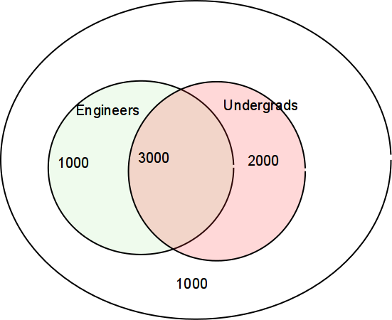
  1. Consider a fictional university that has both undergrads and grads. It also has both Engineers and others:

    /images/venn-stu.png
  2. Compute P[E|U], P[E|U'], P[U|E], etc.

4 Bayes theorem ctd

  1. Wikipedia on Bayes theorem.

    We'll do the defective item example, using both numbers and Bayes rule.

  2. We'll do these examples from Leon-Garcia in class.

  3. Example 2.28, page 51. Assume P[A0]=1/3. P[e]=.1 What is P[A0|B0]?

  4. Example 2.30, page 53, chip quality control: For example 2.28, how long do we have to burn in chips so that the survivors have a 99% probability of being good? p=0.1, a=1/20000.

5 Chapter 2 ctd: Independent events

  1. 2.5 Independent events

    1. \(P[A\cap B] = P[A] P[B]\)

    2. P[A|B] = P[A], P[B|A] = P[B]

  2. A,B independent means that knowing A doesn't help you with B.

  3. Mutually exclusive events w.p.>0 must be dependent.

  4. Example 2.32, page 55.

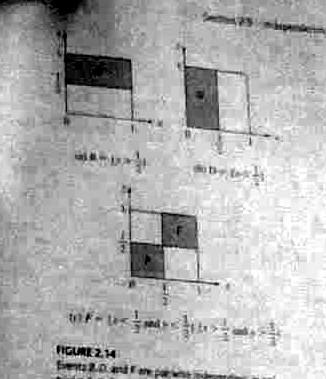
  5. Example 2.33, page 56.

    /images/fig214.jpg
  6. More that 2 events:

    1. N events are independent iff the occurrence of no combo of the events affects another event.

    2. Each pair is independent.

    3. Also need \(P[A\cap B\cap C] = P[A] P[B] P[C]\)

    4. This is not intuitive A, B, and C might be pairwise independent, but, as a group of 3, are dependent.

    5. See example 2.32, page 55. A: x>1/2. B: y>1/2. C: x>y

  7. Common application: independence of experiments in a sequence.

  8. Example 2.34: coin tosses are assumed to be independent of each other.

    P[HHT] = P[1st coin is H] P[2nd is H] P[3rd is T].

  9. Example 2.35, page 58. System reliability

    1. Controller and 3 peripherals.

    2. System is up iff controller and at least 2 peripherals are up.

    3. Add a 2nd controller.

  10. 2.6 p59 Sequential experiments: maybe independent

  11. 2.6.1 Sequences of independent experiments

    1. Example 2.36

  12. 2.6.2 Binomial probability

    1. Bernoulli trial flip a possibly unfair coin once. p is probability of head.

    2. (Bernoulli did stats, econ, physics, ... in 18th century.)

  13. Example 2.37

    1. P[TTH] = \((1-p)^2 p\)

    2. P[1 head] = \(3 (1-p)^2 p\)

  14. Probability of exactly k successes = \(p_n(k) = {n \choose k} p^k (1-p)^{n-k}\)

  15. \(\sum_{k=0}^n p_n(k) = 1\)

  16. Example 2.38

  17. Can avoid computing n! by computing \(p_n(k)\) recursively, or by using approximation. Also, in C++, using double instead of float helps. (Almost always you should use double instead of float. It's the same speed on normal CPUs.)

  18. Example 2.39

  19. Example 2.40 Error correction coding

Engineering Probability Class 6 Thurs 2021-02-11

1 New teaching tool

Today's new gimmick is mirroring my ipad to a window on my laptop, so I can use the ipad as a graphics tablet. Relevant SW: uxplay on the laptop; see https://rodrigoribeiro.site/2020/08/09/mirroring-ipad-iphone-screen-on-linux/ and any notetaking tool on the ipad.

Earlier I tried using a laptop with a touch screen. That didn't work well, apparently because of deficiencies with linux SW controlling the screen.

2 Applied EE

My home Tesla powerwalls (27KHW capacity) and solar panels (8KW peak) are finally working. Over the year, my net electrical consumption will be close to zero. I can survive perhaps a 2-day blackout. However the real reason for getting them is that I like gadgets.

3 Leon Garcia, chapter 2, ctd

  1. 2.4 Conditional probability, page 47.

    1. big topic

    2. E.g., if it snows today, is it more likely to snow tomorrow? next week? in 6 months?

    3. E.g., what is the probability of the stock market rising tomorrow given that (it went up today, the deficit went down, an oil pipeline was blown up, ...)?

    4. What's the probability that a CF bulb is alive after 1000 hours given that I bought it at Walmart?

    5. definition \(P[A|B] = \frac{P[A\cap B]}{P[B]}\)

  2. E.g., if DARPA had been allowed to run its Futures Markets Applied to Prediction (FutureMAP) would the future probability of King Zog I being assassinated be dependent on the amount of money bet on that assassination occurring?

    1. Is that good or bad?

    2. Would knowing that the real Zog survived over 55 assassination attempts change the probability of a future assassination?

  3. Consider a fictional university that has both undergrads and grads. It also has both Engineers and others:

    /images/venn-stu.png
  4. \(P[A\cap B] = P[A|B]P[B] = P[B|A]P[A]\)

  5. Example 2.26 Binary communication. Source transmits 0 with probability (1-p) and 1 with probability p. Receiver errs with probability e. What are probabilities of 4 events?

  6. Total probability theorem

    1. \(B_i\) mutually exclusive events whose union is S

    2. P[A] = P[A \(\cap B_1\) + P[A \(\cap B_2\) + ...

    3. \(P[A] = P[A|B_1]P[B_1]\) \(+ P[A|B_2]P[B_2] + ...\)

    /images/totalprob.png

    What's the probability that a student is an undergrad, given ... (Numbers are fictitious.)

  7. Example 2.28. Chip quality control.

    1. Each chip is either good or bad.

    2. P[good]=(1-p), P[bad]=p.

    3. If the chip is good: P[still alive at t] = \(e^{-at}\)

    4. If the chip is bad: P[still alive at t] = \(e^{-1000at}\)

    5. What's the probability that a random chip is still alive at t?

  8. 2.4.1, p52. Bayes' rule. This lets you invert the conditional probabilities.

    1. \(B_j\) partition S. That means that

      1. If \(i\ne j\) then \(B_i\cap B_j=\emptyset\) and

      2. \(\bigcup_i B_i = S\)

    2. \(P[B_j|A] = \frac{B_j\cap A}{P[A]}\) \(= \frac{P[A|B_j] P[B_j]}{\sum_k P[A|B_k] P[B_k]}\)

    3. application:

      1. We have a priori probs \(P[B_j]\)

      2. Event A occurs. Knowing that A has happened gives us info that changes the probs.

      3. Compute a posteriori probs \(P[B_j|A]\)

  9. In the above diagram, what's the probability that an undergrad is an engineer?

  10. Example 2.29 comm channel: If receiver sees 1, which input was more probable? (You hope the answer is 1.)

  11. Example 2.30 chip quality control: For example 2.28, how long do we have to burn in chips so that the survivors have a 99% probability of being good? p=0.1, a=1/20000.

  12. Example: False positives in a medical test

    1. T = test for disease was positive; T' = .. negative

    2. D = you have disease; D' = .. don't ..

    3. P[T|D] = .99, P[T' | D'] = .95, P[D] = 0.001

    4. P[D' | T] (false positive) = 0.98 !!!

  13. Multinomial probability law

    1. There are M different possible outcomes from an experiment, e.g., faces of a die showing.

    2. Probability of particular outcome: \(p_i\)

    3. Now run the experiment n times.

    4. Probability that i-th outcome occurred \(k_i\) times, \(\sum_{i=1}^M k_i = n\)

      \begin{equation*} P[(k_1,k_2,...,k_M)] = \frac{n!}{k_1! k_2! ... k_M!} p_1^{k_1} p_2^{k_2}...p_M^{k_M} \end{equation*}
  14. Example 2.41 p63 dartboard.

  15. Example 2.42 p63 random phone numbers.

  16. 2.7 Computer generation of random numbers

    1. Skip this section, except for following points.

    2. Executive summary: it's surprisingly hard to generate good random numbers. Commercial SW has been known to get this wrong. By now, they've gotten it right (I hope), so just call a subroutine.

    3. Arizona lottery got it wrong in 1998.

    4. Even random electronic noise is hard to use properly. The best selling 1955 book A Million Random Digits with 100,000 Normal Deviates had trouble generating random numbers this way. Asymmetries crept into their circuits perhaps because of component drift. For a laugh, read the reviews.

    5. Pseudo-random number generator: The subroutine returns numbers according to some algorithm (e.g., it doesn't use cosmic rays), but for your purposes, they're random.

    6. Computer random number routines usually return the same sequence of number each time you run your program, so you can reproduce your results.

    7. You can override this by seeding the generator with a genuine random number from linux /dev/random.

  17. 2.8 and 2.9 p70 Fine points: Skip.

  18. Review Bayes theorem, since it is important. Here is a fictitious (because none of these probilities have any justification) SETI example.

    1. A priori probability of extraterrestrial life = P[L] = \(10^{-8}\).

    2. For ease of typing, let L' be the complement of L.

    3. Run a SETI experiment. R (for Radio) is the event that it has a positive result.

    4. P[R|L] = \(10^{-5}\), P[R|L'] = \(10^{-10}\).

    5. What is P[L|R] ?

  19. Some specific probability laws

    1. In all of these, successive events are independent of each other.

    2. A Bernoulli trial is one toss of a coin where p is probability of head.

    3. We saw binomial and multinomial probilities in class 4.

    4. The binomial law gives the probability of exactly k heads in n tosses of an unfair coin.

    5. The multinomial law gives the probability of exactly ki occurrances of the i-th face in n tosses of a die.

  20. Example 2.28, p51. Chip quality control.

    1. Each chip is either good or bad.

    2. P[good]=(1-p), P[bad]=p.

    3. If the chip is good: P[still alive at t] = \(e^{-at}\)

    4. If the chip is bad: P[still alive at t] = \(e^{-1000at}\)

    5. What's the probability that a random chip is still alive at t?

  21. 2.4.1, p52. Bayes' rule. This lets you invert the conditional probabilities.

    1. \(B_j\) partition S. That means that

      1. If \(i\ne j\) then \(B_i\cap B_j=\emptyset\) and

      2. \(\bigcup_i B_i = S\)

    2. \(P[B_j|A] = \frac{B_j\cap A}{P[A]}\) \(= \frac{P[A|B_j] P[B_j]}{\sum_k P[A|B_k] P[B_k]}\)

    3. application:

      1. We have a priori probs \(P[B_j]\)

      2. Event A occurs. Knowing that A has happened gives us info that changes the probs.

      3. Compute a posteriori probs \(P[B_j|A]\)

  22. In the above diagram, what's the probability that an undergrad is an engineer?

  23. Example 2.29 comm channel: If receiver sees 1, which input was more probable? (You hope the answer is 1.)

  24. Example 2.30 chip quality control: For example 2.28, how long do we have to burn in chips so that the survivors have a 99% probability of being good? p=0.1, a=1/20000.

  25. Example: False positives in a medical test

    1. T = test for disease was positive; T' = .. negative

    2. D = you have disease; D' = .. don't ..

    3. P[T|D] = .99, P[T' | D'] = .95, P[D] = 0.001

    4. P[D' | T] (false positive) = 0.98 !!!

4 Bayes theorem ctd

  1. Wikipedia on Bayes theorem.

    We'll do the examples.

  2. We'll do these examples from Leon-Garcia in class.

  3. Example 2.28, page 51. I'll use e=0.1.

    Variant: Assume that P[A0]=.9. Redo the example.

  4. Example 2.30, page 53, chip quality control: For example 2.28, how long do we have to burn in chips so that the survivors have a 99% probability of being good? p=0.1, a=1/20000.

  5. Event A is that a random person has a lycanthopy gene. Assume P(A) = .01.

    Genes-R-Us has a DNA test for this. B is the event of a positive test. There are false positives and false negatives each w.p. (with probability) 0.1. That is, P(B|A') = P(B' | A) = 0.1

    1. What's P(A')?

    2. What's P(A and B)?

    3. What's P(A' and B)?

    4. What's P(B)?

    5. You test positive. What's the probability you're really positive, P(A|B)?

5 Chapter 2 ctd: Independent events

  1. 2.5 Independent events

    1. \(P[A\cap B] = P[A] P[B]\)

    2. P[A|B] = P[A], P[B|A] = P[B]

  2. A,B independent means that knowing A doesn't help you with B.

  3. Mutually exclusive events w.p.>0 must be dependent.

  4. Example 2.33, page 56.

    /images/fig214.jpg
  5. More that 2 events:

    1. N events are independent iff the occurrence of no combo of the events affects another event.

    2. Each pair is independent.

    3. Also need \(P[A\cap B\cap C] = P[A] P[B] P[C]\)

    4. This is not intuitive A, B, and C might be pairwise independent, but, as a group of 3, are dependent.

    5. See example 2.32, page 55. A: x>1/2. B: y>1/2. C: x>y

  6. Common application: independence of experiments in a sequence.

  7. Example 2.34: coin tosses are assumed to be independent of each other.

    P[HHT] = P[1st coin is H] P[2nd is H] P[3rd is T].

  8. Example 2.35, page 58. System reliability

    1. Controller and 3 peripherals.

    2. System is up iff controller and at least 2 peripherals are up.

    3. Add a 2nd controller.

  9. 2.6 p59 Sequential experiments: maybe independent

  10. 2.6.1 Sequences of independent experiments

    1. Example 2.36

  11. 2.6.2 Binomial probability

    1. Bernoulli trial flip a possibly unfair coin once. p is probability of head.

    2. (Bernoulli did stats, econ, physics, ... in 18th century.)

  12. Example 2.37

    1. P[TTH] = \((1-p)^2 p\)

    2. P[1 head] = \(3 (1-p)^2 p\)

  13. Probability of exactly k successes = \(p_n(k) = {n \choose k} p^k (1-p)^{n-k}\)

  14. \(\sum_{k=0}^n p_n(k) = 1\)

  15. Example 2.38

  16. Can avoid computing n! by computing \(p_n(k)\) recursively, or by using approximation. Also, in C++, using double instead of float helps. (Almost always you should use double instead of float. It's the same speed.)

  17. Example 2.39

  18. Example 2.40 Error correction coding

7 To watch

Rich Radke's Probability Bites:

  1. Binomial and Geometric Practice Problems

  2. Bernoulli's Theorem

  3. Discrete Random Variables

https://www.youtube.com/playlist?list=PLuh62Q4Sv7BXkeKW4J_2WQBlYhKs_k-pj

Engineering Probability Class 5 Mon 2021-02-08

1 TAs

We have two 10-hour TAs:

  1. Heshan Fernando, fernah, office hour: Wednesday 2pm.

  2. Meng Zhang, zhangm19, office hour: Friday 3-4pm.

Their office hours will be on webex, at https://rensselaer.webex.com/meet/RCSID. If no one appears after 15 minutes, they'll leave. OTOH, if you'd like help at other times, contact them. They'll try to be available.

2 Leon Garcia, chapter 2, ctd

  1. Leon-Garcia 2.3: Counting methods, pp 41-46.

    1. finite sample space

    2. each outcome equally probable

    3. get some useful formulae

    4. warmup: consider a multiple choice exam where 1st answer has 3 choices, 2nd answer has 5 choices and 3rd answer has 6 choices.

      1. Q: How many ways can a student answer the exam?

      2. A: 3x5x6

    5. If there are k questions, and the i-th question has \(n_i\) answers then the number of possible combinations of answers is \(n_1n_2 .. n_k\)

  2. 2.3.1 Sampling WITH replacement and WITH ordering

    1. Consider an urn with n different colored balls.

    2. Repeat k times:

      1. Draw a ball.

      2. Write down its color.

      3. Put it back.

    3. Number of distinct ordered k-tuples = \(n^k\)

  3. Example 2.1.5. How many distinct ordered pairs for 2 balls from 5? 5*5.

  4. Review. Suppose I want to eat one of the following 4 places, for tonight and again tomorrow, and don't care if I eat at the same place both times: Commons, Sage, Union, Knotty Pine. How many choices to I have where to eat?

    1. 16

    2. 12

    3. 8

    4. 4

    5. something else

  5. 2.3.2 Sampling WITHOUT replacement and WITH ordering

    1. Consider an urn with n different colored balls.

    2. Repeat k times:

      1. Draw a ball.

      2. Write down its color.

      3. Don't put it back.

    3. Number of distinct ordered k-tuples = n(n-1)(n-2)...(n-k+1)

  6. Review. Suppose I want to visit two of the following four cities: Buffalo, Miami, Boston, New York. I don't want to visit one city twice, and the order matters. How many choices to I have how to visit?

    1. 16

    2. 12

    3. 8

    4. 4

    5. something else

  7. Example 2.1.6: Draw 2 balls from 5 w/o replacement.

    1. 5 choices for 1st ball, 4 for 2nd. 20 outcomes.

    2. Probability that 1st ball is larger?

    3. List the 20 outcomes. 10 have 1st ball larger. P=1/2.

  8. Example 2.1.7: Draw 3 balls from 5 with replacement. What's the probability they're all different?

    1. P = \(\small \frac{\text{# cases where they're different}}{\text{# cases where I don't care}}\)

    2. P = \(\small \frac{\text{# case w/o replacement}}{\text{# cases w replacement}}\)

    3. P = \(\frac{5*4*3}{5*5*5}\)

  9. 2.3.3 Permutations of n distinct objects

    1. Distinct means that you can tell the objects apart.

    2. This is sampling w/o replacement for k=n

    3. 1.2.3.4...n = n!

    4. It grows fast. 1!=1, 2!=2, 3!=6, 4!=24, 5!=120, 6!=720, 7!=5040

    5. Stirling approx:

      \begin{equation*} n! \approx \sqrt{2\pi n} \left(\frac{n}{e}\right)^n\left(1+\frac{1}{12n}+...\right) \end{equation*}
    6. Therefore if you ignore the last term, the relative error is about 1/(12n).

  10. Example 2.1.8. # permutations of 3 objects. 6!

  11. Example 2.1.9. 12 airplane crashes last year. Assume independent, uniform, etc, etc. What's probability of exactly one in each month?

    1. For each crash, let the outcome be its month.

    2. Number of events for all 12 crashes = \(12^{12}\)

    3. Number of events for 12 crashes in 12 different months = 12!

    4. Probability = \(12!/(12^{12}) = 0.000054\)

    5. Random does not mean evenly spaced.

  12. 2.3.4 Sampling w/o replacement and w/o ordering

    1. We care what objects we pick but not the order

    2. E.g., drawing a hand of cards.

    3. term: Combinations of k objects selected from n. Binomial coefficient.

      \begin{equation*} C^n_k = {n \choose k} = \frac{n!}{k! (n-k)!} \end{equation*}
    4. Permutations is when order matters.

  13. Example 2.20. Select 2 from 5 w/o order. \(5\choose 2\)

  14. Example 2.21 # permutations of k black and n-k white balls. This is choosing k from n.

  15. Example 2.22. 10 of 50 items are bad. What's probability 5 of 10 selected randomly are bad?

    1. # ways to have 10 bad items in 50 is \(50\choose 10\)

    2. # ways to have exactly 5 bad is 3 ways to select 5 good from 40 times # ways to select 5 bad from 10 = \({40\choose5} {10\choose5}\)

    3. Probability is ratio.

  16. Multinomial coefficient: Partition n items into sets of size \(k_1, k_2, ... k_j, \sum k_i=n\)

    \begin{equation*} \frac{n!}{k_1! k_2! ... k_j!} \end{equation*}
  17. 2.3.5. skip

Reading: 2.4 Conditional probability, page 47-

  1. New stuff, pp. 47-66:

    1. Conditional probability - If you know that event A has occurred, does that change the probability that event B has occurred?

    2. Independence of events - If no, then A and B are independent.

    3. Sequential experiments - Find the probability of a sequence of experiments from the probabilities of the separate steps.

    4. Binomial probabilities - tossing a sequence of unfair coins.

    5. Multinomial probabilities - tossing a sequence of unfair dice.

    6. Geometric probabilities - toss a coin until you see the 1st head.

    7. Sequences of dependent experiments - What you see in step 1 influences what you do in step 2.

3 To watch

Rich Radke's Probability Bites:

  1. The Monty Hall Problem

  2. Independent Events

  3. Bernoulli Trials

https://www.youtube.com/playlist?list=PLuh62Q4Sv7BXkeKW4J_2WQBlYhKs_k-pj

4 Occasional no-work classes

Since there is no spring break, or even many long weekends, occasionally the probability class will be something easy, with no homework and no exam questions, like watching a video.

5 Probability in the real world - enrichment

See examples in the random section below.

6 Homework 3

is online here , due in a week.

Engineering Probability Class 4 Thurs 2021-02-04

1 Our various computer systems don't talk to each other

Everyone in this class should--

  1. be in gradescope,

  2. have received an invitation to webex meet for the lectures,

  3. be reading the messages in webex (formerly called webex teams),

  4. be in LMS,

  5. be reading this blog.

If you're not in gradescope or webex or webex meet, e.g. because you added late, tell WRF.

3 Chapter 2 ctd

  1. Today: counting methods, Leon-Garcia section 2.3, page 41.

    1. We have an urn with n balls.

    2. Maybe the balls are all different, maybe not.

    3. W/o looking, we take k balls out and look at them.

    4. Maybe we put each ball back after looking at it, maybe not.

    5. Suppose we took out one white and one green ball. Maybe we care about their order, so that's a different case from green then white, maybe not.

  2. Applications:

    1. How many ways can we divide a class of 12 students into 2 groups of 6?

    2. How many ways can we pick 4 teams of 6 students from a class of 88 students (leaving 64 students behind)?

    3. We pick 5 cards from a deck. What's the probability that they're all the same suit?

    4. We're picking teams of 12 students, but now the order matters since they're playing baseball and that's the batting order.

    5. We have 100 widgets; 10 are bad. We pick 5 widgets. What's the probability that none are bad? Exactly 1? More than 3?

    6. In the approval voting scheme, you mark as many candidates as you please. The candidate with the most votes wins. How many different ways can you mark the ballot?

    7. In preferential voting, you mark as many candidates as you please, but rank them 1,2,3,... How many different ways can you mark the ballot?

4 To watch

Rich Radke's Probability Bites:

  1. The Total Probability Theorem

  2. Bayes' Rule

  3. A Medical Testing Example

https://www.youtube.com/playlist?list=PLuh62Q4Sv7BXkeKW4J_2WQBlYhKs_k-pj

6 Future homework format

Instead of having a big homework every week, we'll have smaller homeworks after every class, due in several days. The total work will be the same, but this will test you on the material more quickly. The questions will generally be multiple choice.

Engineering Probability Class 3 Mon 2021-02-01

1 Homework 2

is online, due in a week.

3 Chapter 2 ctd

  1. Corollory 6:

    \(\begin{array}{c} P\left[\cup_{i=1}^n A_i\right] = \\ \sum_{i=1}^n P[A_i] \\ - \sum_{i<j} P[A_i\cap A_j] \\ + \sum_{i<j<k} P[A_i\cap A_j\cap A_k] \cdots \\ + (-1)^{n+1} P[\cap_{i=1}^n A_i] \end{array}\)

    1. Example Q=queen card, H=heart, F= face card.

      1. P[Q]=4/52, P[H]=13/52, P[F]=12/52,

      2. P[Q \(\cap\) H]=1/52, P[Q \(\cap\) F] = ''you tell me''

      3. P[H \(\cap\) F]= ''you tell me''

      4. P[Q \(\cap\) H \(\cap\) F] = ''you tell me''

      5. So P[Q \(\cup\) H \(\cup\) F] = ?

    2. Example from Roulette:

      1. R=red, B=black, E=even, A=1-12

      2. P[R] = P[B] = P[E] = 16/38. P[A]=12/38

      3. \(P[R\cup E \cup A]\) = ?

  2. Corollory 7: if \(A\subset B\) then P[A] <= P[B]

    Example: Probability of a repeated coin toss having its first head in the 2nd-4th toss (1/2+1/4+1/8) \(\ge\) Probability of it happening in the 3rd toss (1/4).

  3. 2.2.1 Discrete sample space

    1. If sample space is finite, probabilities of all the outcomes tell you everything.

    2. sometimes they're all equal.

    3. Then P[event]} \(= \frac{\text{#. outcomes in event}}{\text{total # outcomes}}\)

    4. For countably infinite sample space, probabilities of all the outcomes also tell you everything.

    5. E.g. fair coin. P[even] = 1/2

    6. E.g. example 2.9. Try numbers from random.org.

    7. What probabilities to assign to outcomes is a good question.

    8. Example 2.10. Toss coin 3 times.

      1. Choice 1: outcomes are TTT ... HHH, each with probability 1/8

      2. Choice 2: outcomes are # heads: 0...3, each with probability 1/4.

      3. Incompatible. What are probabilities of # heads for choice 1?

      4. Which is correct?

      5. Both might be mathematically ok.

      6. It depends on what physical system you are modeling.

      7. You might try doing the experiment and observing.

      8. You might add a new assumption: The coin is fair and the tosses independent.

  4. Example 2.11: countably infinite sample space.

    1. Toss fair coin, outcome is # tosses until 1st head.

    2. What are reasonable probabilities?

    3. Do they sum to 1?

  5. 2.2.2 Continuous sample spaces

    1. Usually we can't assign probabilities to points on real line. (It just doesn't work out mathematically.)

    2. Work with set of intervals, and Boolean operations on them.

    3. Set may be finite or countable.

    4. This set of events is a ''Borel set''.

    5. Notation:

      1. [a,b] closed. includes both. a<=x<=b

      2. (a,b) open. includes neither. a<x<b

      3. [a,b) includes a but not b, a<=x<b

      4. (a,b] includes b but not a, a<x<=b

    6. Assign probabilities to intervals (open or closed).

    7. E.g., uniform distribution on [0,1] \(P[a\le x\le b] = \frac{1}{b-a}\)

    8. Nonuniform distributions are common.

    9. Even with a continuous sample space, a few specific points might have probabilities. The following is mathematically a valid probability distribution. However I can't immediately think of a physical system that it models.

      1. \(S = \{ x | 0\le x\le 1 \}\)

      2. \(p(x=1) = 1/2\)

      3. For \(0\le x_0 \le 1, p(x<x_0) = x_0/2\)

  6. For fun: Heads you win, tails... you win. You can beat the toss of a coin and here's how....

  7. Example 2.13, page 39, nonuniform distribution: chip lifetime.

    1. Propose that P[(t, \(\infty\) )] = \(e^{-at}\) for t>0.

    2. Does this satisfy the axioms?

    3. I: yes >0

    4. II: yes, P[S] = \(e^0\) = 1

    5. III here is more like a definition for the probability of a finite interval

    6. P[(r,s)] = P[(r, \(\infty\) )] - P[(s, \(\infty\) )] = \(e^{-ar} - e^{-as}\)

  8. Probability of a precise value occurring is 0, but it still can occur, since SOME value has to occur.

  9. Example 2.14: picking 2 numbers randomly in a unit square.

    1. Assume that the probability of a point falling in a particular region is proportional to the area of that region.

    2. E.g. P[x>1/2 and y<1/10] = 1/20

    3. P[x>y] = 1/2

  10. Recap:

    1. Problem statement defines a random experiment

    2. with an experimental procedure and set of measurements and observations

    3. that determine the possible outcomes and sample space

    4. Make an initial probability assignment

    5. based on experience or whatever

    6. that satisfies the axioms.

4 To watch

Rich Radke's Probability Bites:

  1. Combinatorics Practice Problems

  2. Continuous Sample Spaces

  3. Conditional Probability

https://www.youtube.com/playlist?list=PLuh62Q4Sv7BXkeKW4J_2WQBlYhKs_k-pj

PROB Engineering Probability Homework 2 due Mon 2021-02-08

Submit the answers to Gradescope.

OK to work in teams of 2. Form a gradescope group and submit once for the team.

Questions

  1. (6 pts) Do exercise 2.2, page 81 of Leon-Garcia.

  2. (6 pts) Do exercise 2.4, page 81.

  3. (6 pts) Do exercise 2.6, page 82.

  4. (6 pts) Do exercise 2.21, page 84.

  5. (6 pts) Do exercise 2.25, page 84.

  6. (6 pts) Do exercise 2.35(a), page 85. Assume the "half as frequently" means that for a subinterval of length d, the probability is half as much when the subinterval is in [0,2] as when in [-1,0).

  7. (6 pts) Do exercise 2.39, page 86. Ignore any mechanical limitations of combo locks. Good RPI students should know what those limitations are.

    (Aside: A long time ago, RPI rekeyed the whole campus with a more secure lock. Shortly thereafter a memo was distributed that I would summarize as, "OK, you can, but don't you dare!")

  8. (6 pts) Do exercise 2.59, page 87. However, make it 21 students and 3 on each day of the week. Assume that there is no relation between birthday and day of the week.

  9. (6 pts) Find a current policy issue where you think that probabilities are being misused, and say why, in 100 words. Full points will be awarded for a logical argument. I don't care what the issue is, or which side you take. Try not to pick something too too inflammatory; follow the Page 1 rule that an NSF lawyer taught me when I worked there as a Program Director for a few years. (Would you be willing to see your answer on page 1 of tomorrow's paper?)

Total: 54 pts.

Engineering Probability Class 2 Thu 2021-01-28

2 Probability in the real world - enrichment

  1. How Did Economists Get It So Wrong? is an article by Paul Krugman (2008 Nobel Memorial Prize in Economic Science). It says, "the economics profession went astray because economists, as a group, mistook beauty, clad in impressive-looking mathematics, for truth." You might see a certain relevance to this course. You have to get the model right before trying to solve it.

    Though I don't know much about it, I'll cheerfully try to answer any questions about econometrics.

    Another relevance to this course, in an enrichment sense, is that some people believe that the law of large numbers does not apply to certain variables, like stock prices. They think that larger and larger sample frequencies do not converge to a probability, because the variance of the underlying distribution is infinite. This also is beyond this course.

3 Chapter 1 ctd

  1. Rossman-Chance coin toss applet demonstrates how the observed frequencies converge (slowly) to the theoretical probability.

  2. Example of unreliable channel (page 12)

    1. Want to transmit a bit: 0, 1

    2. It arrives wrong with probability e, say 0.001

    3. Idea: transmit each bit 3 times and vote.

      1. 000 -> 0

      2. 001 -> 0

      3. 011 -> 1

    1. 3 bits arrive correct with probability \((1-e)^3\) = 0.997002999

    2. 1 error with probability \(3(1-e)^2e\) = 0.002994

    3. 2 errors with probability \(3(1-e)e^2\) = 0.000002997

    4. 3 errors with probability \(e^3\) = 0.000000001

    5. corrected bit is correct if 0 or 1 errors, with probability \((1-e)^3+3(1-e)^2e\) = 0.999996999

    6. We reduced probability of error by factor of 1000.

    7. Cost: triple the transmission plus a little logic HW.

  3. Example of text compression (page 13)

    1. Simple way: Use 5 bits for each letter: A=00000, B=00001

    2. In English, 'E' common, 'Q' rare

    3. Use fewer bits for E than Q.

    4. Morse code did this 170 years ago.

      1. E = .

      2. Q = _ _ . _

    1. Aside: An expert Morse coder is faster than texting.

    2. English can be compressed to about 1 bit per letter (with difficulty); 2 bits is easy.

    3. Aside: there is so much structure in English text, that if you add the bit strings for 2 different texts bit-by-bit, they can usually mostly be reconstructed.

    4. That's how cryptoanalysis works.

  4. Example of reliable system design (page 13)

    1. Nuclear power plant fails if

      1. water leaks

      2. and operator asleep (a surprising number of disasters happen in the graveyard shift).

      3. and backup pump fails

      4. or was turned off for maintenance

    1. What's the probability of failure? This depends on the probabilities of the various failure modes. Those might be impossible to determine accurately.

    2. Design a better system? Coal mining kills.

    3. The backup procedures themselves can cause problems (and are almost impossible to test). A failure with the recovery procedure was part of the reason for a Skype outage.

4 Chapter 2

  1. A random experiment (page 21) has 2 parts:

    1. experimental procedure

    2. set of measurements

  2. Random experiment may have subexperiments and sequences of experiments.

  3. Outcome or sample point \(\zeta\): a non-decomposable observation.

  4. Sample space S: set of all outcomes

  5. \(|S|\):

    1. finite, e.g. {H,T}, or

    2. discrete = countable, e.g., 1,2,3,4,... Sometimes discrete includes finite. or

    3. uncountable, e.g., \(\Re\), aka continuous.

  6. Types of infinity:

    1. Some sets have finite size, e.g., 2 or 6.

    2. Other sets have infinite size.

    3. Those are either countable or uncountable.

    4. A countably infinite set can be arranged in order so that its elements can be numbered 1,2,3,...

    5. The set of natural numbers is obviously countable.

    6. The set of positive rational numbers between 0 and 1 is also countable. You can order it thus: \(\frac{1}{1}, \frac{1}{2}, \frac{1}{3}, \frac{2}{3}, \frac{1}{4}, \ \frac{3}{4}, \frac{1}{5}, \frac{2}{5}, \frac{3}{5}, \ \cdots\)

    7. The set of real numbers is not countable (aka uncountable). Proving this is beyond this course. (It uses something called diagonalization.

    8. Uncountably infinite is a bigger infinity than countably infinite, but that's beyond this course.

    9. Georg Cantor, who formulated this, was hospitalized in a mental health facility several times.

  7. Why is this relevant to probability?

    1. We can assign probabilities to discrete outcomes, but not to individual continuous outcomes.

    2. We can assign probabilities to some events, or sets of continuous outcomes.

  8. E.g. Consider this experiment to watch an atom of sodium-26.

    1. Its half-life is 1 second (Applet: Nuclear Isotope Half-lifes)

    2. Define the outcomes to be the number of complete seconds before it decays: \(S=\{0, 1, 2, 3, \cdots \}\)

    3. \(|S|\) is countably infinite, i.e., discrete.

    4. \(p(0)=\frac{1}{2}, p(1)=\frac{1}{4}, \cdots\) \(p(k)=2^{-(k+1)}\)

    5. \(\sum_{k=0}^\infty p(k) = 1\)

    6. We can define events like these:

      1. The atom decays within the 1st second. p=.5.

      2. The atom decays within the first 3 seconds. p=.875.

      3. The atom's lifetime is an even number of seconds. \(p = \frac{1}{2} + \frac{1}{8} + \frac{1}{32} + \cdots = \frac{2}{3}\)

  9. Now consider another experiment: Watch another atom of Na-26

    1. But this time the outcome is defined to be the real number, x, that is the time until it decays.

    2. \(S = \{ x | x\ge0 \}\)

    3. \(|S|\) is uncountably infinite.

    4. We cannot talk about the probability that x=1.23 exactly. (It just doesn't work out.)

    5. However, we can define the event that \(1.23 < x < 1.24\), and talk about its probability.

    6. \(P[x>x_0] = 2^{-x_0}\)

    7. \(P[1.23 < x < 1.24]\) \(= 2^{-1.23} - 2^{-1.24} = 0.003\)

  10. Event

    1. collection of outcomes, subset of S

    2. what we're interested in.

    3. e.g., outcome is voltage, event is V>5.

    4. certain event: S

    5. null event: \(\emptyset\)

    6. elementary event: one discrete outcome

  11. Set theory

    1. Sets: S, A, B, ...

    2. Universal set: U

    3. elements or points: a, b, c

    4. \(a\in S, a\notin S\), \(A\subset B\)

    5. Venn diagram

    6. empty set: {} or \(\emptyset\)

    7. operations on sets: equality, union, intersection, complement, relative complement

    8. properties (axioms): commutative, associative, distributive

    9. theorems: de Morgan

  12. Prove deMorgan 2 different ways.

    1. Use the fact that A equals B iff A is a subset of B and B is a subset of A.

    2. Look at the Venn diagram; there are only 4 cases.

  13. 2.1.4 Event classes

    1. Remember: an event is a set of outcomes of an experiment, e.g., voltage.

    2. In a continuous sample space, we're interested only in some possible events.

    3. We're interested in events that we can measure.

    4. E.g., we're not interested in the event that the voltage is exactly an irrational number.

    5. Events that we're interested in are intervals, like [.5,.6] and [.7,.8].

    6. Also unions and complements of intervals.

    7. This matches the real world. You can't measure a voltage as 3.14159265...; you measure it in the range [3.14,3.15].

    8. Define \(\cal F\) to be the class of events of interest: those sets of intervals.

    9. We assign probabilities only to events in \(\cal F\).

  14. 2.2 Axioms of probability

    1. An axiom system is a general set of rules. The probability axioms apply to all probabilities.

    2. Axioms start with common sense rules, but get less obvious.

    3. I: 0<=P[A]

    4. II: P[S]=1

    5. III: \(A\cap B=\emptyset \rightarrow\) \(P[A\cup B] = P[A]+P[B]\)

    6. III': For \(A_1, A_2, ....\) if \(\forall_{i\ne j} A_i \cap A_j = \emptyset\) then \(P[\bigcup_{i=1}^\infty A_i]\) \(= \sum_{i=1}^\infty P[A_i]\)

  15. Example: cards. Q=event that card is queen, H=event that card is heart. These events are not disjoint. Probabilities do not sum.

    1. \(Q\cap H \ne\emptyset\)

    2. P[Q] = 1/13=4/52, P[H] = 1/4=13/52, P[Q \(\cup\) H] = 16/52!=17/52.

  16. Example C=event that card is clubs. H and C are disjoint. Probabilities do sum.

    1. \(C\cap H = \emptyset\).

    2. P[C] = 13/52, P[H] = 1/4=13/52, P[Q \(\cup\) H] = 26/52.

  17. Example. Flip a fair coin \(A_i\) is the event that the first time you see heads is the i-th time, for \(i\ge1\).

    1. We can assign probabilities to these countably infinite number of events.

    2. \(P[A_i] = 1/2^i\)

    3. They are disjoint, so probabilities sum.

    4. Probability that the first head occurs in the 10th or later toss = \(\sum_{i=10}^\infty 1/2^i\)

  18. Corollory 1

    1. \(P[A^c] = 1-P[A]\)

    2. E.g., P[heart] = 1/4, so P[not heart] = 3/4

  19. Corollory 2: P[A] <=1

  20. Corollory 3: P[\(\emptyset\)] = 0

  21. Corollory 4:

    1. For \(A_1, A_2, .... A_n\) if \(\forall_{i\ne j} A_i \cap A_j = \emptyset\) then \(P\left[\bigcup_{i=1}^n A_i\right] = \sum_{i=1}^n P[A_i]\)

    2. Proof by induction from axiom III.

  22. Prove de Morgan's law (page 28)

  23. Corollory 5 (page 33): \(P[A\cup B] = P[A] + P[B] - P[A\cap B]\)

    1. Example: Queens and hearts. P[Q]=4/52, P[H]=13/52, P[Q \(\cup\) H]=16/52, P[Q \(\cap\) H]=1/52.

    2. \(P[A\cup B] \le P[A] + P[B]\)

5 Questions

Continuous probability:

  1. S is the real interval [0,1].

  2. P([a,b]) = b-a if 0<=a<=b<=1.

  3. Event A = [.2,.6].

  4. Event B = [.4,1].

Questions:

  1. What is P[A]?

    1. .2

    2. .4

    3. .6

    4. .8

  2. What is P[B]?

    1. .2

    2. .4

    3. .6

    4. .8

  3. What is P[A \(\cup\) B]?

    1. .2

    2. .4

    3. .6

    4. .8

  4. What is P[A \(\cap\) B]?

    1. .2

    2. .4

    3. .6

    4. .8

  5. What is P[A \(\cup\) B \(^c\) ]?

    1. .2

    2. .4

    3. .6

    4. .8

  6. Retransmitting a noisy bit 3 times: Set e=0.1. What is probability of no error in 3 bits:

    1. 0.1

    2. 0.3

    3. 0.001

    4. 0.729

    5. 0.9

  7. Flipping a fair coin until we get heads: How many times will it take until the probability of seeing a head is >=.8?

    1. 1

    2. 2

    3. 3

    4. 4

    5. 5

  8. This time, the coin is weighted so that p[H]=.6. How many times will it take until the probability of seeing a head is >=.8?

    1. 1

    2. 2

    3. 3

    4. 4

    5. 5

7 To read

Leon-Garcia, chapter 2.

8 To watch

Rich Radke's Probability Bites:

  1. Axioms of Probability

  2. Discrete Sample Spaces

  3. Combinatorics

https://www.youtube.com/playlist?list=PLuh62Q4Sv7BXkeKW4J_2WQBlYhKs_k-pj

PROB Engineering Probability Syllabus, S2021

This is the syllabus for ENGR-2500 Engineering Probability, Rensselaer Polytechnic Institute, Spring 2021.

1 Catalog description

ENGR-2500 Engineering Probability

Axioms of probability, joint and conditional probability, random variables, probability density, mass, and distribution functions, functions of one and two random variables, characteristic functions, sequences of independent random variables, central limit theorem, and laws of large numbers. Applications to electrical and computer engineering problems.

Prerequisites/Corequisites: Corequisite: ECSE 2410.

When Offered: Fall and spring terms annually.

Credit Hours: 3.

2 Course Goals / Objectives

To understand basic probability theory and statistical analysis and be able to apply them to modeling typical computer and electrical engineering problems such as noisy signals, decisions in the presence of uncertainty, pattern recognition, network traffic, and digital communications.

3 Student Learning Outcomes

Students will be able to:

  1. Be able to apply basic probability theory.

  2. Be able to apply concepts of probability to model typical computer and electrical engineering problems.

  3. Be able to evaluate the performance of engineering systems with uncertainty.

4 Instructors

4.1 Professor

W. Randolph Franklin. BSc (Toronto), AM, PhD (Harvard)

Office

virtual

Phone

+1 (518) 276-6077 (forwards)

Email

frankwr@YOUKNOWTHEDOMAIN

Email is my preferred communication medium.

Web

https://wrf.ecse.rpi.edu/

A quick way to get there is to google RPIWRF.

Office hours

After each lecture, usually as long as anyone wants to talk. Also by appointment.

Informal meetings

If you would like to talk with me, either individually or in a group, just mention it. We can then talk about most anything legal and ethical.

4.2 Teaching assistants

  1. Who:

    1. Heshan Fernando <fernah@THEUSUAL>,

    2. Meng Zhang <zhangm19@THEUSUAL>

  2. Office hours:

    1. Webex teams (probably)

    2. times TBD

  3. They will try to stay as long as there are students asking questions, but will leave after 15 minutes if no one has arrived.

  4. If you need more time, or a different time, then write them.

5 Identifying yourself in email

If you use a non-RPI email account, please make your name part of the address, so, when I scan my inbox, it's obvious who the sender is. Tagging the subject with #Prob is also helpful. So is including your RCSID in the message. Your RCSID is letters and possibly numbers, not nine digits. Mine is FRANKWR.

6 Computer usage

6.1 Course wiki

This current page https://wrf.ecse.rpi.edu/Teaching/probability-s2021/ has lecture summaries, syllabus, homeworks, etc. You can also get to it from my home page.

6.2 Piazza

I don't intend to use piazza.

6.3 Gradescope

Gradescope will be used for you to submit homeworks and for us to distribute grades.

6.4 Webex meetings

We'll start by using this for classes.

6.5 Webex teams

Use this for discussions and asking questions.

6.6 Matlab

Matlab may be used for computations.

6.7 Mathematica

I will use Mathematica for examples. You are not required to know or to use it, although you're welcome to. Mathematica handles formulae.

7 Textbooks etc

  1. Leon-Garcia, Probability, Statistics, and Random Processes for Electrical Engineering, 3rd Ed., Pearson/Prentice-Hall, 2008. ISBN 978-0-13-147122-1.

    Why I picked it (in spite of the price, which keeps increasing each year):

    1. It is a good book.

    2. This is the same book as we've used for several years.

    3. This book is used at many other universities because it is good. Those courses' lecture notes are sometimes online, if you care to look.

  2. There is also a lot of web material on probability. Wikipedia is usually good.

8 Class times & places

  1. Mon & Thurs, 3:00- 4:20PM, Online.

  2. Probability will be completely virtual. I intend to lecture live, with some supplementary videos. Students will be encouraged to ask questions with chat during the class. I'll try to save it, but the chat window might be deleted after each class. If you cannot watch the class live, then you may miss any info presented in the chat window.

  3. I will maintain a class blog that briefly summarizes each class. Important points will be written down. See https://wrf.ecse.rpi.edu/Teaching/probability-s2021/ .

  4. I will attempt to record all classes and upload them to mediasite for students to watch or download later. However, this fall, about 10% of classes failed to record properly. If this happens, then you will miss that class.

  5. There will be no class attendance taken. Any in-class quizzes will not be graded.

  6. Therefore, if you are in a far away time zone, you should do ok.

  7. How exams including the final exam will occur will be decided later.

  8. In general, if the conflicting class is not in ECSE, then I expect you to treat my class more seriously, e.g., attend it live more often. FYI, Probability's time was changed to avoid a conflict with another ECSE class.

  9. I intend no class activities outside the scheduled times, except for a possible final exam review, a day or two before the exam.

  10. Except when some equipment fails, I post an copy of everything that I write in class.

  11. I welcome short questions that have short answers.

  12. I will usually stay after class so long as anyone wants to meet me.

9 Assessment measures, i.e., grades

You are welcome to put copies of exams and homeworks in test banks, etc, if they are free to access. However since I put everything online, it's redundant.

9.1 Exams

  1. There will be a total of three exams of which the two best count towards the final grade.

  2. Dates and details tbd. However I realize that some students are many time zones away.

  3. There are no make-up exams, as the one of the exams can be dropped.

  4. If you're satisfied with your first two exam grades, then you may skip the final.

9.2 Homework

  1. Homework will be assigned frequently, perhaps after most classes.

  2. Submit your completed homework assignments in Gradescope by midnight on the due date.

  3. Late homeworks receive a 50% reduction of the points if the homework is less than 24hrs late.

  4. Homeworks will not be accepted more than 24hrs late except in cases of an excused absences.

  5. Homework keys will be posted.

  6. The homework sets can be done in groups of up to two students.

  7. The make-up of the groups is allowed to change from one homework set to the next.

  8. Each member of a group working on a homework set will receive the same grade for this homework.

  9. Some homework questions will be recycled as exam questions.

  10. We will drop the lowest homework.

9.3 Bonus knowitall points

  1. You can earn an extra point by giving me a pointer to interesting material on the web, good enough to post on the class wiki.

  2. Occasionally I make mistakes, either in class or on the web site. The first person to correct each nontrival error will receive an extra point on his/her grade.

  3. One person may accumulate several of these knowitall points.

9.4 Weights and cutoffs

Relative weights of the different grade components

Component

Weight

All the homeworks together

30%

Top 2 of the 3 exams (each)

35%

Even if the homeworks be out of different numbers of points, they will be normalized so that each homework has the same weight, except that the lowest homework will be dropped.

Grade cutoffs:

Percentage grade

Letter grade

>=95.0%

A

>=90.0%

A-

>=85.0%

B+

>=80.0%

B

>=75.0%

B-

>=70.0%

C+

>=65.0%

C

>=60.0%

C-

>=55.0%

D+

>=50.0%

D

>=0%

F

However, if that causes the class average to be lower than the prof and TAs feel that the class deserves, based on how hard students appeared to work, then the criteria will be eased.

9.5 Grade distribution & verification

  1. We'll post homework grading comments on Gradescope.

  2. If you disagree with a grade, then

    1. report it within one week,

    2. in writing,

    3. emailed to a TA, with a copy to the prof.

  3. It is not allowed to wait until the end of the semester, and then go back 3 months to try to find extra points.

  4. We maintain standards (and the value of your diploma) by giving the grades that are earned, not the grades that are desired. Nevertheless, this course's average grade is competitive with other courses.

  5. If you feel that you have been treated unfairly, appeal in writing, first to a TA, then to the prof, to another prof acting as mediator if you wish, and then to the ECSE Head.

9.6 Mid-semester assessment

After the first exam and before the drop date, we will compute an estimate of your performance to date.

9.7 Early warning system (EWS)

As required by the Provost, we may post notes about you to EWS, for example, if you're having trouble doing homeworks on time, or miss an exam. E.g., if you tell me that you had to miss a class because of family problems, then I may forward that information to the Dean of Students office.

10 Academic integrity

  1. See the Student Handbook for the general policy. The summary is that students and faculty have to trust each other. After you graduate, your most important possession will be your reputation.

Specifics for this course are as follows.

  1. You may collaborate on homeworks, but each team people must write up the solution separately (one writeup per team) using their own words. We willingly give hints to anyone who asks.

  2. The penalty for two teams handing in identical work is a zero for both.

  3. Writing assistance from the Writing Center and similar sources in allowed, if you acknowledge it.

  4. The penalty for plagiarism is a zero grade.

  5. You must not communicate with other people or machines, exchange notes, or use electronic aids like computers and PDAs during exams.

  6. The penalty is a zero grade on the exam.

  7. Cheating will be reported to the Dean of Students Office.

11 Other RPI rules

You've seen them in your other classes. They're incorporated here by reference.

12 Students with special accommodations

Please send me your authorizing memo.

13 Student feedback

Since it's my desire to give you the best possible course in a topic I enjoy teaching, I welcome feedback during (and after) the semester. You may tell me or write me or the TAs, or contact a third party, such as Prof John Wen, the ECSE Dept head.

PROB Engineering Probability Class 1 Mon 2020-01-13

1 Topics

  1. Syllabus and Intro.

  2. Why probability is useful

    1. AT&T installed bandwidth to provide level of iphone service (not all users want to use it simultaneously).

    2. also web servers, roads, cashiers, ...

    3. What is a fair price for a car or health or life insurance?

    4. Will a pension plan go broke?

    5. What would you pay today for the right to buy a share of Tesla (TSLA) on 6/30/20 for 400 dollars? (Today, 1/10/19, it is 478.) The answer is not simply $78. It is complicated because you don't have to buy if TSLA is below $400 then.

  3. To model something

    1. Real thing too expensive, dangerous, time-consuming (aircraft design).

    2. Capture the relevant, ignore the rest.

    3. Coin flip: relevant: it's fair? not relevant: copper, tin, zinc, ...

    4. Validate model if possible.

  4. Computer simulation model

    1. For systems too complicated for a simple math equation (i.e., most systems outside school)

    2. Often a graph of components linked together, e.g., with

      1. Matlab Simulink

      2. PSPICE

    1. many examples, e.g. antilock brake, US economy

    2. Can do experiments on it.

  5. To make public policy: "Compas (Correctional Offender Management Profiling for Alternative Sanctions), is used throughout the U.S. to weigh up whether defendants awaiting trial or sentencing are at too much risk of reoffending to be released on bail." Slashdot.

  6. Deterministic model

    1. Resistor: V=IR

    2. Limitations: perhaps not if I=1000000 amps. Why?

    3. Limitations: perhaps not if I=0.00000000001 amps. Why?

  7. Probability model

    1. Roulette wheel: \(p_i=\frac{1}{38}\) (ignoring http://www.amazon.com/Eudaemonic-Pie-Thomas-Bass/dp/0595142362 )

  8. Terms

    1. Random experiment: different outcomes each time it's run.

    2. Outcome: one possible result of a random experiment.

    3. Sample space: set of possible outcomes.

      1. Discrete, or

      2. Continuous.

    1. Tree diagram of successive discrete experiments.

    2. Event: subset of sample space.

    3. Venn diagram: graphically shows relations.

  9. Statistical regularity

    1. \(lim_{n\rightarrow\infty}f_k(n) =p_k\)

    2. law of large numbers

    3. weird distributions (e.g., Cauchy) violate this, but that's probably beyond this course.

  10. Properties of relative frequency

    1. the frequencies of all the possibilities sum to 1.

    2. if an event is composed of several outcomes that are disjoint, the event's probability is the sum of the outcomes' probabilities.

    3. E.g., If the event is your passing this course and the relevant outcomes are grades A, B, C, D, with probabilities .3, .3, .2, .1, then \(p_{pass}=0.9\) . (These numbers are fictitious.)

  11. Axiomatic approach

    1. Probability is between 0 and 1.

    2. Probs sum to 1.

    3. If the events are disjoint, then the probs add.

  12. Building a model

    1. Want to model telephone conversations where speaker talks 1/3 of time.

    2. Could use an urn with 2 black, 1 white ball.

    3. Computer random number generator easier.

  13. Detailed example in more detail - phone system

    1. Design telephone system for 48 simultaneous users.

    2. Transmit packet of voice every 10msecs.

    3. Only 1/3 users are active.

    4. 48 channels wasteful.

    5. Alloc only M<48 channels.

    6. In the next 10msec block, A people talked.

    7. If A>M, discard A-M packets.

    8. How good is this?

    9. n trials

    10. \(N_k(n)\) trials have k packets

    11. frequency \(f_k(n)=N_k(n)/n\)

    12. \(f_k(n)\rightarrow p_k\) probability

    13. We'll see the exact formula (Poisson) later.

    14. average number of packets in one interval:

      \(\frac{\sum_{k=1}^{48} kN_k(n)}{n} \rightarrow \sum_{k=1}^{48} kp_k = E[A]\)

    15. That is the expected value of A.

  14. Probability application: unreliable communication channel.

    1. Transmitter transmits 0 or 1.

    2. Receiver receives 0 or 1.

    3. However, a transmitted 0 is received as a 0 only 90% of the time, and

    4. a transmitted 1 is received as a 1 only 80% of the time, so

    5. if you receive a 0 what's the probability that a 0 was transmitted?

    6. ditto 1.

    7. (You don't have enough info to answer this; you need to know also the probability that a 0 was transmitted. Perhaps the transmitter always sends a 0.)

  15. Another application: stocking spare parts:

    1. There are 10 identical lights in the classroom ceiling.

    2. The lifetime of each bulb follows a certain distribution. Perhaps it dies uniformly anytime between 1000 and 3000 hours.

    3. As soon as a light dies, the janitor replaces it with a new one.

    4. How many lights should the janitor stock so that there's a 90% chance that s/he won't run out within 5000 hours?

2 To read

Leon-Garcia, chapter 1.

3 To watch

Rich Radke's Probability Bites:

  1. Introduction

  2. Experiments and Sample Spaces

  3. Events

https://www.youtube.com/playlist?list=PLuh62Q4Sv7BXkeKW4J_2WQBlYhKs_k-pj

PROB Engineering Probability Homework 1 due Mon 2021-02-01

Submit the answers to Gradescope.

Questions

  1. (7 pts) One of the hardest problems is forming an appropriate probability model. E.g., suppose you're working for Verizon deciding how much data capacity your network will need once it starts selling the iphone. Suppose that you know that each customer will use 10GB/month. Since a month has about 2.5M seconds, does that mean that your network will need to provide only 4KB/s per customer? What might be wrong with this model? How might you make it better? (This is an open-ended question; any reasonable answer that shows creativity gets full points.)

  2. (7 pts) One hard problem with statistics is how they should be interpreted. For example, mental health care professionals observe that young men with schizophrenia are usually pot (marijuana) smokers. Assuming for the sake of argument that this correlation is real, does this mean that pot smoking causes schizophrenia?

    Historical note: In 1974, the question of whether cigarette smoking causes lung cancer was answered by forcing some dogs in a lab to smoke and observing that they got cancer more than otherwise identical dogs forced to not smoke.

    The tobacco companies were maintaining that the strong correlation between smoking and lung cancer (1/4 of smokers died from cancer, and almost everyone who died from lung cancer was a smoker) did not demonstrate a causal relation. Maybe there was a common cause for both a desire to smoke and a likelihood to later get cancer. These experiments refuted that claim.

    Mary Beith, the journalist who broke the 'smoking beagles' story

    https://i.guim.co.uk/img/static/sys-images/Guardian/Pix/pictures/2012/5/20/1337511110598/phpn42MCJAM.jpg?width=620&quality=45&auto=format&fit=max&dpr=2&s=f5b5fadc7c650d2db5cae1e60e6d7c18
  3. (12 pts) Do exercise 1.1 (a-b for each of 3 experiments) in the text on page 18.

  4. (12 pts) Do exercise 1.5 (a-c) on page 19.

  5. (12 pts) Do exercise 1.10 (a-c) on page 20.

Total: 50 pts.