1   Chapter 3 ctd

1. Geometric distribution: review mean and variance.

2. Suppose that you have just sold your internet startup for $10M. You have retired and now you are trying to climb Mt Everest. You intend to keep trying until you make it. Assume that:

   1. Each attempt has a 1/3 chance of success.
   2. The attempts are independent; failure on one does not affect future attempts.
   3. Each attempt costs $70K.

   Iclicker: What is your expected cost of a successful climb?

   1. $70K.
   2. $140K.
   3. $210K.
   4. $280K.
   5. $700K.

3. 3.4 page 111 Conditional pmf

4. Example 3.24 Residual waiting time

   1. X, time to xmit message, is uniform in 1...L.
   2. If X is over m, what's probability that remaining time is j?
   3. \(p_X(m+j|X>m) = \frac{P[X =m+j]}{P[X>m]} = \frac{1/L}{(L-m)/L} = 1/(L-m)\)

5. \(p_X(x) = \sum p_X(x|B_i) P[B_i]\)

6. Example 3.25 p 113 device lifetimes

   1. 2 classes of devices, geometric lifetimes.
   2. Type 1, probability \(\alpha\), parameter r. Type 2 parameter s.
   3. What's pmf of the total set of devices?

7. Example 3.26.

8. 3.5 More important discrete r.v

9. Table 3.1: We haven't seen \(G_X(z)\) yet.

10. 3.5.4 Poisson r.v.

    1. The experiment is observing how many of a large number of rare events happen in, say, 1 minute.

    2. E.g., how many cosmic particles hit your DRAM, how many people call to call center.

    3. The individual events are independent. (In the real world this might be false. If a black hole occurs, you're going to get a lot of cosmic particles. If the ATM network crashes, there will be a lot of calls.)

    4. The r.v. is the number that happen in that period.

    5. There is one parameter, \(\alpha\). Often this is called \(\lambda\).

       \begin{equation*} p(k) = \frac{\alpha^k}{k!}e^{-\alpha} \end{equation*}

    6. Mean and std dev are both \(\alpha\).

    7. In the real world, events might be dependent.

1   Iclicker questions

1. Imagine that the coin you toss might land on its edge (and stay there). P(head)=.5, p(tail)=.4, p(edge)=.1. You toss it 3 times. What's the probability that it lands on its head twice, and on edge once?
   1. .025
   2. .05
   3. .075
   4. .081
   5. .1
2. Now you toss the coin repeatedly until it lands on edge. What's the probability that this happens for the first time on the 3rd toss?
   1. .025
   2. .05
   3. .081
   4. .1
   5. .333
3. iClicker: You have a coin where the probability of a head is p=2/3 What's the probability that the 1st head occurs on the 2nd toss?
   1. 1/2
   2. 1/3
   3. 2/9
   4. 5/9
   5. 4/9

2   Wikipedia

Wikipedia's articles on technical subjects can be excellent. In fact, they often have more detail than you want. Here are some that are relevant to this course. Read at least the first few paragraphs.

1. https://en.wikipedia.org/wiki/Outcome_(probability)
2. https://en.wikipedia.org/wiki/Random_variable
3. https://en.wikipedia.org/wiki/Indicator_function
4. https://en.wikipedia.org/wiki/Gambler%27s_fallacy
5. https://en.wikipedia.org/wiki/Fat-tailed_distribution
6. https://en.wikipedia.org/wiki/St._Petersburg_paradox

3   Two types of testing errors

1. There's an event A, with probability P[A]=p.
2. There's a dependent event, perhaps a test or a transmission, B.
3. You know P[B|A] and P[B|A'].
4. Wikipedia:
   1. https://en.wikipedia.org/wiki/Type_I_and_type_II_errors
   2. https://en.wikipedia.org/wiki/Sensitivity_and_specificity
5. Terminology:
   1. Type I error, False negative.
   2. Type II error, false positive.
   3. Sensitivity, true positive proportion.
   4. Selectivity, true negative proportion.

4   Chapter 3 ctd

1. This chapter covers Discrete (finite or countably infinite) r.v.. This contrasts to continuous, to be covered later.
2. Discrete r.v.s we've seen so far:
   1. uniform: M events 0...M-1 with equal probs
   2. bernoulli: events: 0 w.p. q=(1-p) or 1 w.p. p
   3. binomial: # heads in n bernoulli events
   4. geometric: # trials until success, each trial has probability p.
3. 3.1.1 Expected value of a function of a r.v.
   1. Z=g(X)
   2. E[Z] = E[g(x)] = \(\sum_k g(x_k) p_X(x_k)\)
4. Example 3.17 square law device
5. \(E[a g(X)+b h(X)+c] = a E[g(X)] + b E[h(x)] + c\)
6. Example 3.18 Square law device continued
7. Example 3.19 Multiplexor discards packets
8. Compute mean of a binomial distribution.
9. Compute mean of a geometric distribution.
10. 3.3.1, page 107: Operations on means: sums, scaling, functions
11. iclicker: From a deck of cards, I draw a card, look at it, put it back and reshuffle. Then I do it again. What's the probability that exactly one of the 2 cards is a heart?
    • A: 2/13
    • B: 3/16
    • C: 1/4
    • D: 3/8
    • E: 1/2
12. iclicker: From a deck of cards, I draw a card, look at it, put it back and reshuffle. I keep repeating this. What's the probability that the 2nd card is the 1st time I see hearts?
    • A: 2/13
    • B: 3/16
    • C: 1/4
    • D: 3/8
    • E: 1/2
13. 3.3.2 page 109 Variance of an r.v.
    1. That means, how wide is its distribution?
    2. Example: compare the performance of stocks vs bonds from year to year. The expected values (means) of the returns may not be so different. (This is debated and depends, e.g., on what period you look at). However, stocks' returns have a much larger variance than bonds.
    3. \(\sigma^2_X = VAR[X] = E[(X-m_X)^2] = \sum (x-m_x)^2 p_X(x)\)
    4. standard deviation \(\sigma_X = \sqrt{VAR[X]}\)
    5. \(VAR[X] = E[X^2] - m_X^2\)
    6. 2nd moment: \(E[X^2]\)
    7. also 3rd, 4th... moments, like a Taylor series for probability
    8. shifting the distribution: VAR[X+c] = VAR[X]
    9. scaling: \(VAR[cX] = c^2 VAR[X]\)
14. Derive variance for Bernoulli.
15. Example 3.20 3 coin tosses
    1. general rule for binomial: VAR[X]=npq
    2. Derive it.
    3. Note that it sums since the events are independent.
    4. Note that variance/mean shrinks as n grows.
16. iclicker: The experiment is drawing a card from a deck, seeing if it's hearts, putting it back, shuffling, and repeating for a total of 100 times. The random variable is the total # of hearts seen, from 0 to 100. What's the mean of this r.v.?
    • A: 1/4
    • B: 25
    • C: 1/2
    • D: 50
    • E: 1
17. iclicker: The experiment is drawing a card from a deck, seeing if it's hearts, putting it back, shuffling, and repeating for a total of 100 times. The random variable is the # of hearts seen, from 0 to 100. What's the variance of this r.v.?
    • A: 3/16
    • B: 1
    • C: 25/4
    • D: 75/4
    • E: 100

1   Iclicker questions

1. Imagine that the coin you toss might land on its edge (and stay there). P(head)=.5, p(tail)=.4, p(edge)=.1. You toss it 3 times. What's the probability that it lands on its head twice, and on edge once?
   1. .025
   2. .05
   3. .081
   4. .1
   5. .333
2. Now you toss the coin repeatedly until it lands on edge. What's the probability that this happens for the first time on the 3rd toss?
   1. .025
   2. .05
   3. .081
   4. .1
   5. .333

2   Chapter 2 ctd

1. 2.6.4 p63 Geometric probability law

   1. Repeat Bernoulli experiment until 1st success.
   2. Define outcome to be # trials until that happens.
   3. Define q=(1-p).
   4. \(p(m) = (1-p)^{m-1}p = q^{m-1}p\) (p has 2 different uses here).
   5. \(\sum_{m=1}^\infty p(m) =1\)
   6. Probability that more than K trials are required = \(q^K\).

2. Example: probability that more than 10 tosses of a die are required to get a 6 = \(\left(\frac{5}{6}\right)^{10} = 0.16\)

3. iClicker: You have a coin where the probability of a head is p=2/3 What's the probability that the 1st head occurs on the 2nd toss?

   1. 1/2
   2. 1/3
   3. 2/9
   4. 5/9
   5. 4/9

4. Example 2.43: error control by retransmission. A sent over a noisy channel is checksummed so the receiver can tell if it got mangled, and then ask for retransmission. TCP/IP does this.

   Aside: This works better when the roundtrip time is reasonable. Using this when talking to Mars is challenging.

5. 2.6.5 p64 Sequences, chains, of dependent experiments.

   1. This is an important topic, but mostly beyond this course.
   2. In many areas, there are a sequence of observations, and the probability of each observation depends on what you observed before.
   3. It relates to Markov chains.
   4. Motivation: speech and language recognition, translation, compression
   5. E.g., in English text, the probability of a u is higher if the previous char was q.
   6. The probability of a b may be higher if the previous char was u (than if it was x), but is lower if the previous two chars are qu.
   7. Need to look at probabilities of sequences, char by char.
   8. Same idea in speech recognition: phonemes follow phonemes...
   9. Same in language understanding: verb follows noun...

6. Example 2.44, p64

   1. In this example, you repeatedly choose an urn to draw a ball from, depending on what the previous ball was.

3   Discrete Random Variables

1. Chapter 3, p 96. Discrete random variables
   1. From now on our random experiments will always produce numbers, called random variables, at least indirectly.
   2. Then we can compute, e.g., a fair value to pay for a gamble. What should you pay to play roulette so that betting on red breaks even on average?
   3. Discrete is different from discreet.
   4. Random experiment \(\rightarrow\) nonnumerical outcome \(\zeta\) \(\rightarrow\)
   5. Random Variable \(X(\zeta )\). Any real number.
   6. Random vars in general: X, Y, ...
   7. particular values: x, y, ...
   8. It's the outcome that's random, not the r.v., which is a deterministic function of the outcome.
2. Example 3.1 Coin tosses
   1. Define X to be the number of heads from 3 tosses.
   2. \(\zeta\)
3. Example 3.2 Betting game addon to 3.1
   1. Define another random var Y to be payoff: 8 if X=3, 1 if X=2, 0 else.
   2. Y is derived from X
4. Example 3.3 add probs to 3.2, assuming fair coin. P[X=2], P[Y=8]
5. 3.1.1 Ignore since it's starred.
6. 3.2 Discrete r.v. and Probability mass function (pmf).
   1. The pmf shows the probability of every value of random variable X, and of every real number.
   2. If X cannot have the value x, then the pmf is 0 at x.
   3. \(p_X(x) = P[X=x] = P[\{\zeta:X(\zeta)=x\}]\)
7. p100: 3 properties of pmf. They're all common sense.
   1. Nonnegative.
   2. Sums to one.
   3. The probability of an event B is the sum of the probabilities of the outcomes in B.
8. Example 3.5 probability of # heads in 3 coin tosses: \(p_X(0)=1/8\)
9. Example 3.6 betting game \(p_Y(1)=3/8\)
10. Fig 3.4. You can graph the pmf.
11. There are many types of random variables, depending on the shape of the pmf. These start out the same as the various probability laws in Chapter 2. However we'll see more types (e.g., Poisson) and more properties of each type (e.g., mean, standard deviation, generating function).
12. Example 3.7 random number generator
    1. produces integer X equally likely in range 0..M-1
    2. \(S_X=\{0, 1, ... M-1 \}\)
    3. pmf: \(p_X(k)=1/M\) for k in 0..M-1.
    4. X is a uniform random variable over that set.
13. Example 3.8 Bernoulli random variable
    1. indicator function \(I_A(\zeta)=1\) iff \(\zeta\in A\)
    2. pmf of \(I_A\): \(p_I(0)=1-p, p_I(1)=p\)
    3. \(I_A\) is a Bernoulli random variable.
14. Example 3.9 Message transmission until success
    1. \(p_X(k)=q^{k-1}p, k=1,2,3,...\)
    2. Geometric random variable
    3. What about P[X is even]?
15. Example 3.10 Number of transmission errors
    1. \(p_X(k) = {n \choose k} p^k q^{n-k}, k=0,1,...n\)
    2. binomial random variable
16. Fig 3.5 You can graph the relative frequencies from running an experiment repeatedly.
    1. It will approach the pmf graph (absent pathological cases like the Cauchy distribition that are beyond this course.)
17. 3.3 p104 Expected value and other moments
    1. This is a way to summarize a r.v., and capture important aspects.
    2. E.g., What's a fair price to pay for a lottery ticket?
    3. Mean or expected value or center of mass: \(m_X = E[X] = \sum_{x\in S_X} x p_X(x)\)
    4. Defined iff absolute convergence: \(\sum |x| p(x) < \infty\)
18. Example 3.11 Mean of Bernoulli r.v.
19. Example 3.12 Mean of Binomial r.v. What's the expected # of heads in 3 tosses?
20. Example 3.13 Mean of uniform discrete r.v.
21. Run an experiment n times and observe \(x(1), x(2), ...\)
    1. \(N_k(n)\) # times \(x_k\) was seen
    2. \(f_k(n) = N_k(n)/n\) frequencies
    3. Sample mean \(<X>_n = \sum x_kf_k(n)\)
    4. With lots of experiments, frequencies approach probabilities and sample mean converges to E[X]
    5. However it may take a long time, which is why stock market investors can go broke first.
22. Example 3.14 p 106 Betting game
23. Example 3.15 Mean of a geometric r.v.
24. Example 3.16 St Petersburg paradox

1   Bayes theorem ctd

1. Wikipedia on Bayes theorem. We'll do these examples in class.
2. Example 2.28, page 51.
3. Example 2.30, page 53, chip quality control: For example 2.28, how long do we have to burn in chips so that the survivors have a 99% probability of being good? p=0.1, a=1/20000.

2   Iclicker review of Bayes theorem

1. Event A is that a random person has a lycanthopy gene. Assume P(A) = .01.

   Genes-R-Us has a DNA test for this. B is the event of a positive test. There are false positives and false negatives each w.p. (with probability) 0.1. That is, P(B|A') = P(B' | A) = 0.1

   What's P(A')?

   1. 0.09
   2. .099
   3. .189
   4. .48
   5. .99

2. What's P(A and B)?

   1. 0.09
   2. .099
   3. .189
   4. .48
   5. .99

3. What's P(A' and B)?

   1. 0.09
   2. .099
   3. .189
   4. .48
   5. .99

4. What's P(B)?

   1. 0.09
   2. .099
   3. .189
   4. .48
   5. .99

5. You test positive. What's the probability you're really positive, P(A|B)?

   1. 0.09
   2. .099
   3. .189
   4. .48
   5. .99

3   Chapter 2 ctd: Independent eventa

1. 2.5 Independent events

   1. \(P[A\cap B] = P[A] P[B]\)
   2. P[A|B] = P[A], P[B|A] = P[B]

2. A,B independent means that knowing A doesn't help you with B.

3. Mutually exclusive events w.p.>0 must be dependent.

4. Example 2.33, page 56.

   

5. More that 2 events:

   1. N events are independent iff the occurrence of no combo of the events affects another event.
   2. Each pair is independent.
   3. Also need \(P[A\cap B\cap C] = P[A] P[B] P[C]\)
   4. This is not intuitive A, B, and C might be pairwise independent, but, as a group of 3, are dependent.
   5. See example 2.32, page 55. A: x>1/2. B: y>1/2. C: x>y

6. Common application: independence of experiments in a sequence.

7. Example 2.34: coin tosses are assumed to be independent of each other.

   P[HHT] = P[1st coin is H] P[2nd is H] P[3rd is T].

8. Example 2.35, page 58. System reliability

   1. Controller and 3 peripherals.
   2. System is up iff controller and at least 2 peripherals are up.
   3. Add a 2nd controller.

9. 2.6 p59 Sequential experiments: maybe independent

10. 2.6.1 Sequences of independent experiments

    1. Example 2.36

11. 2.6.2 Binomial probability

    1. Bernoulli trial flip a possibly unfair coin once. p is probability of head.
    2. (Bernoulli did stats, econ, physics, ... in 18th century.)

12. Example 2.37

    1. P[TTH] = \((1-p)^2 p\)
    2. P[1 head] = \(3 (1-p)^2 p\)

13. Probability of exactly k successes = \(p_n(k) = {n \choose k} p^k (1-p)^{n-k}\)

14. \(\sum_{k=0}^n p_n(k) = 1\)

15. Example 2.38

16. Can avoid computing n! by computing \(p_n(k)\) recursively, or by using approximation. Also, in C++, using double instead of float helps. (Almost always you should use double instead of float. It's the same speed.)

17. Example 2.39

18. Example 2.40 Error correction coding

19. Multinomial probability law

    1. There are M different possible outcomes from an experiment, e.g., faces of a die showing.

    2. Probability of particular outcome: \(p_i\)

    3. Now run the experiment n times.

    4. Probability that i-th outcome occurred \(k_i\) times, \(\sum_{i=1}^M k_i = n\)

       \begin{equation*} P[(k_1,k_2,...,k_M)]` :math:`= \frac{n!}{k_1! k_2! ... k_M!} p_1^{k_1} p_2^{k_2}...p_M^{k_M} \end{equation*}

20. Example 2.41 dartboard.

21. Example 2.42 random phone numbers.

22. 2.7 Computer generation of random numbers

    1. Skip this section, except for following points.
    2. Executive summary: it's surprisingly hard to generate good random numbers. Commercial SW has been known to get this wrong. By now, they've gotten it right (I hope), so just call a subroutine.
    3. Arizona lottery got it wrong in 1998.
    4. Even random electronic noise is hard to use properly. The best selling 1955 book A Million Random Digits with 100,000 Normal Deviates had trouble generating random numbers this way. Asymmetries crept into their circuits perhaps because of component drift. For a laugh, read the reviews.
    5. Pseudo-random number generator: The subroutine returns numbers according to some algorithm (e.g., it doesn't use cosmic rays), but for your purposes, they're random.
    6. Computer random number routines usually return the same sequence of number each time you run your program, so you can reproduce your results.
    7. You can override this by seeding the generator with a genuine random number from linux /dev/random.

23. 2.8 and 2.9 p70 Fine points: Skip.

24. Review Bayes theorem, since it is important. Here is a fictitious (because none of these probilities have any justification) SETI example.

    1. A priori probability of extraterrestrial life = P[L] = \(10^{-8}\).
    2. For ease of typing, let L' be the complement of L.
    3. Run a SETI experiment. R (for Radio) is the event that it has a positive result.
    4. P[R|L] = \(10^{-5}\), P[R|L'] = \(10^{-10}\).
    5. What is P[L|R] ?

25. Some specific probability laws

    1. In all of these, successive events are independent of each other.
    2. A Bernoulli trial is one toss of a coin where p is probability of head.
    3. We saw binomial and multinomial probilities in class 4.
    4. The binomial law gives the probability of exactly k heads in n tosses of an unfair coin.
    5. The multinomial law gives the probability of exactly ki occurrances of the i-th face in n tosses of a die.

26. iClicker: You have a coin where the probability of a head is p=2/3 If you toss it twice, what's the probability that you will see one head and one tail?

    1. 1/2
    2. 1/3
    3. 2/9
    4. 5/9
    5. 4/9

How to submit

Submit to LMS; see details in syllabus.

Questions

1. (5 points) Assume that it is known that one person in a group of 100 committed a crime. You're in the group, so there's a prior probability of 1/100 that you are it. There is a pretty good forensic test. It makes errors (either way) only 0.1% of the time. You are given the test; the result is positive. Using this positive test, what's the probability now that you are the criminal? (Use Bayes.)
2. 5. Do exercise 2.59, page 87. However, make it 21 students and 3 on each day of the week. Assume that there is no relation between birthday and day of the week.
3. (5 pts) Do exercise 2.62 on page 88 of the text.
4. (5 pts) Do 2.69, but use the interval [-2,2].
5. (5 pts) Do 2.72.
6. (5 pts) Do 2.76.
7. (5 pts) Do 2.82.
8. (5 pts) Do 2.97.
9. (5 pts) Do 2.102.
10. (5 pts) Do 2.106.

Total: 50 pts.

1   Iclicker review

1. Followon to the meal choice iclicker question. My friend and I wish to visit a hospital, chosen from: Memorial, AMC, Samaritan. We might visit different hospitals.
   1. If we don't care whether we visit the same hospital or not, in how many ways can we do this?
      1. 1
      2. 2
      3. 3
      4. 6
      5. 9
   2. We wish to visit different hospitals, to later write a Poly review. In how many ways can we visit different hospitals, where we care which hospital each of us visits?
      1. 1
      2. 2
      3. 3
      4. 6
      5. 9
   3. Modify the above, to say that we care only about the set of hospitals we two visit.
      1. 1
      2. 2
      3. 3
      4. 6
      5. 9
   4. We realize that Samaritan and Memorial are both owned by St Peters and we want to visit two different hospital chains to write our reviews. In how many ways can we pick hospitals so that we pick different chains?
      1. 1
      2. 2
      3. 3
      4. 4
      5. 5
   5. We each pick between Memorial and AMC with 50% probability, independently. What is the probability that each hospital is picked exactly once (in contrast to picking one twice and the other not at all).
      1. 0
      2. 1/4
      3. 1/2
      4. 3/4
      5. 1

2   Chapter 2 ctd

1. New stuff, pp. 47-66:

   1. Conditional probability - If you know that event A has occurred, does that change the probability that event B has occurred?
   2. Independence of events - If no, then A and B are independent.
   3. Sequential experiments - Find the probability of a sequence of experiments from the probabilities of the separate steps.
   4. Binomial probabilities - tossing a sequence of unfair coins.
   5. Multinomial probabilities - tossing a sequence of unfair dice.
   6. Geometric probabilities - toss a coin until you see the 1st head.
   7. Sequences of dependent experiments - What you see in step 1 influences what you do in step 2.

2. 2.4 Conditional probability, page 47.

   1. big topic
   2. E.g., if it snows today, is it more likely to snow tomorrow? next week? in 6 months?
   3. E.g., what is the probability of the stock market rising tomorrow given that (it went up today, the deficit went down, an oil pipeline was blown up, ...)?
   4. What's the probability that a CF bulb is alive after 1000 hours given that I bought it at Walmart?
   5. definition \(P[A|B] = \frac{P[A\cap B]}{P[B]}\)

3. E.g., if DARPA had been allowed to run its Futures Markets Applied to Prediction (FutureMAP) would the future probability of King Zog I being assassinated be dependent on the amount of money bet on that assassination occurring?

   1. Is that good or bad?
   2. Would knowing that the real Zog survived over 55 assassination attempts change the probability of a future assassination?

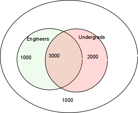
4. Consider a fictional university that has both undergrads and grads. It also has both Engineers and others:

   

5. iClicker: What's the probability that a student is an Engineer?

   1. 1/7
   2. 4/7
   3. 5/7
   4. 3/4
   5. 3/5

6. iClicker: What's the probability that a student is an Engineer, given that s/he is an undergrad?

   1. 1/7
   2. 4/7
   3. 5/7
   4. 3/4
   5. 3/5

7. \(P[A\cap B] = P[A|B]P[B] = P[B|A]P[A]\)

8. Example 2.26 Binary communication. Source transmits 0 with probability (1-p) and 1 with probability p. Receiver errs with probability e. What are probabilities of 4 events?

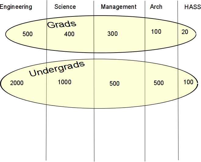
9. Total probability theorem

   1. \(B_i\) mutually exclusive events whose union is S
   2. P[A] = P[A \(\cap B_1\) + P[A \(\cap B_2\) + ...
   3. \(P[A] = P[A|B_1]P[B_1]\) \(+ P[A|B_2]P[B_2] + ...\)
   

   What's the probability that a student is an undergrad, given ... (Numbers are fictitious.)

10. Example 2.28. Chip quality control.

    1. Each chip is either good or bad.
    2. P[good]=(1-p), P[bad]=p.
    3. If the chip is good: P[still alive at t] = \(e^{-at}\)
    4. If the chip is bad: P[still alive at t] = \(e^{-1000at}\)
    5. What's the probability that a random chip is still alive at t?

11. 2.4.1, p52. Bayes' rule. This lets you invert the conditional probabilities.

    1. \(B_j\) partition S. That means that
       1. If \(i\ne j\) then \(B_i\cap B_j=\emptyset\) and
       2. \(\bigcup_i B_i = S\)
    2. \(P[B_j|A] = \frac{B_j\cap A}{P[A]}\) \(= \frac{P[A|B_j] P[B_j]}{\sum_k P[A|B_k] P[B_k]}\)
    3. application:
       1. We have a priori probs \(P[B_j]\)
       2. Event A occurs. Knowing that A has happened gives us info that changes the probs.
       3. Compute a posteriori probs \(P[B_j|A]\)

12. In the above diagram, what's the probability that an undergrad is an engineer?

13. Example 2.29 comm channel: If receiver sees 1, which input was more probable? (You hope the answer is 1.)

14. Example 2.30 chip quality control: For example 2.28, how long do we have to burn in chips so that the survivors have a 99% probability of being good? p=0.1, a=1/20000.

15. Example: False positives in a medical test

    1. T = test for disease was positive; T' = .. negative
    2. D = you have disease; D' = .. don't ..
    3. P[T|D] = .99, P[T' | D'] = .95, P[D] = 0.001
    4. P[D' | T] (false positive) = 0.98 !!!

1   Handwritten notes from class

here

E.g., 117.pdf

2   Chapter 2 ctd

1. Today: counting methods, Leon-Garcia section 2.3, page 41.

   1. We have an urn with n balls.
   2. Maybe the balls are all different, maybe not.
   3. W/o looking, we take k balls out and look at them.
   4. Maybe we put each ball back after looking at it, maybe not.
   5. Suppose we took out one white and one green ball. Maybe we care about their order, so that's a different case from green then white, maybe not.

2. Applications:

   1. How many ways can we divide a class of 12 students into 2 groups of 6?
   2. How many ways can we pick 4 teams of 6 students from a class of 88 students (leaving 64 students behind)?
   3. We pick 5 cards from a deck. What's the probability that they're all the same suit?
   4. We're picking teams of 12 students, but now the order matters since they're playing baseball and that's the batting order.
   5. We have 100 widgets; 10 are bad. We pick 5 widgets. What's the probability that none are bad? Exactly 1? More than 3?
   6. In the approval voting scheme, you mark as many candidates as you please. The candidate with the most votes wins. How many different ways can you mark the ballot?
   7. In preferential voting, you mark as many candidates as you please, but rank them 1,2,3,... How many different ways can you mark the ballot?

3. Leon-Garcia 2.3: Counting methods, pp 41-46.

   1. finite sample space
   2. each outcome equally probable
   3. get some useful formulae
   4. warmup: consider a multiple choice exam where 1st answer has 3 choices, 2nd answer has 5 choices and 3rd answer has 6 choices.
      1. Q: How many ways can a student answer the exam?
      2. A: 3x5x6
   5. If there are k questions, and the i-th question has \(n_i\) answers then the number of possible combinations of answers is \(n_1n_2 .. n_k\)

4. 2.3.1 Sampling WITH replacement and WITH ordering

   1. Consider an urn with n different colored balls.
   2. Repeat k times:
      1. Draw a ball.
      2. Write down its color.
      3. Put it back.
   3. Number of distinct ordered k-tuples = \(n^k\)

5. Example 2.1.5. How many distinct ordered pairs for 2 balls from 5? 5*5.

6. iClicker. Suppose I want to eat one of the following 4 places, for tonight and again tomorrow, and don't care if I eat at the same place both times: Commons, Sage, Union, Knotty Pine. How many choices to I have where to eat?

   1. 16
   2. 12
   3. 8
   4. 4
   5. something else

7. 2.3.2 Sampling WITHOUT replacement and WITH ordering

   1. Consider an urn with n different colored balls.
   2. Repeat k times:
      1. Draw a ball.
      2. Write down its color.
      3. Don't put it back.
   3. Number of distinct ordered k-tuples = n(n-1)(n-2)...(n-k+1)

8. iClicker. Suppose I want to visit two of the following four cities: Buffalo, Miami, Boston, New York. I don't want to visit one city twice, and the order matters. How many choices to I have how to visit?

   1. 16
   2. 12
   3. 8
   4. 4
   5. something else

9. Example 2.1.6: Draw 2 balls from 5 w/o replacement.

   1. 5 choices for 1st ball, 4 for 2nd. 20 outcomes.
   2. Probability that 1st ball is larger?
   3. List the 20 outcomes. 10 have 1st ball larger. P=1/2.

10. Example 2.1.7: Draw 3 balls from 5 with replacement. What's the probability they're all different?

    1. P = \(\small \frac{\text{# cases where they're different}}{\text{# cases where I don't care}}\)
    2. P = \(\small \frac{\text{# case w/o replacement}}{\text{# cases w replacement}}\)
    3. P = \(\frac{5*4*3}{5*5*5}\)

11. 2.3.3 Permutations of n distinct objects

    1. Distinct means that you can tell the objects apart.

    2. This is sampling w/o replacement for k=n

    3. 1.2.3.4...n = n!

    4. It grows fast. 1!=1, 2!=2, 3!=6, 4!=24, 5!=120, 6!=720, 7!=5040

    5. Stirling approx:

       \begin{equation*} n! \approx \sqrt{2\pi n} \left(\frac{n}{e}\right)^n\left(1+\frac{1}{12n}+...\right) \end{equation*}

    6. Therefore if you ignore the last term, the relative error is about 1/(12n).

12. Example 2.1.8. # permutations of 3 objects. 6!

13. Example 2.1.9. 12 airplane crashes last year. Assume independent, uniform, etc, etc. What's probability of exactly one in each month?

    1. For each crash, let the outcome be its month.
    2. Number of events for all 12 crashes = \(12^{12}\)
    3. Number of events for 12 crashes in 12 different months = 12!
    4. Probability = \(12!/(12^{12}) = 0.000054\)
    5. Random does not mean evenly spaced.

14. 2.3.4 Sampling w/o replacement and w/o ordering

    1. We care what objects we pick but not the order

    2. E.g., drawing a hand of cards.

    3. term: Combinations of k objects selected from n. Binomial coefficient.

       \begin{equation*} C^n_k = {n \choose k} = \frac{n!}{k! (n-k)!} \end{equation*}

    4. Permutations is when order matters.

15. Example 2.20. Select 2 from 5 w/o order. \(5\choose 2\)

16. Example 2.21 # permutations of k black and n-k white balls. This is choosing k from n.

17. Example 2.22. 10 of 50 items are bad. What's probability 5 of 10 selected randomly are bad?

    1. # ways to have 10 bad items in 50 is \(50\choose 10\)
    2. # ways to have exactly 5 bad is 3 ways to select 5 good from 40 times # ways to select 5 bad from 10 = \({40\choose5} {10\choose5}\)
    3. Probability is ratio.

18. Multinomial coefficient: Partition n items into sets of size \(k_1, k_2, ... k_j, \sum k_i=n\)

    \begin{equation*} \frac{n!}{k_1! k_2! ... k_j!} \end{equation*}

19. 2.3.5. skip

20. More state lottery incompetence: Statistician Cracks Code For Lottery Tickets

    Finding these stories is just too easy.

Reading: 2.4 Conditional probability, page 47-

3   Iclicker questions

1. Retransmitting a very noisy bit 2 times: The probability of each bit going bad is 0.4. What is probability of no error at all in the 2 transmissions?
   1. 0.16
   2. 0.4
   3. 0.36
   4. 0.48
   5. 0.8
2. Flipping an unfair coin 2 times: The probability of each toss being heads is 0.4. What is probability of both tosses being tails?
   1. 0.16
   2. 0.4
   3. 0.36
   4. 0.48
   5. 0.8
3. Flipping a fair coin until we get heads: How many times will it take until the probability of seeing a head is >=.8?
   1. 1
   2. 2
   3. 3
   4. 4
   5. 5
4. This time, the coin is weighted so that p[H]=.6. How many times will it take until the probability of seeing a head is >=.8?
   1. 1
   2. 2
   3. 3
   4. 4
   5. 5

How to submit

Submit to LMS; see details in syllabus.

Questions

1. (6 pts) Do exercise 2.2, page 81 of Leon-Garcia.

2. (6 pts) Do exercise 2.4, page 81.

3. (6 pts) Do exercise 2.6, page 82.

4. (6 pts) Do exercise 2.21, page 84.

5. (6 pts) Do exercise 2.25, page 84.

6. (6 pts) Do exercise 2.35(a), page 85. Assume the "half as frequently" means that for a subinterval of length d, the probability is half as much when the subinterval is in [0,2] as when in [-1,0).

7. (6 pts) Do exercise 2.39, page 86. Ignore any mechanical limitations of combo locks. Good RPI students should know what those limitations are.

   (Aside: A long time ago, RPI rekeyed the whole campus with a more secure lock. Shortly thereafter a memo was distributed that I would summarize as, "OK, you can, but don't you dare!")

8. (6 pts) Do exercise 2.59, page 87. However, make it 35 students and 3 on each day of the week. Assume that there is no relation between birthday and day of the week.

9. (6 pts) Find a current policy issue where you think that probabilities are being misused, and say why, in 100 words. Full points will be awarded for a logical argument. I don't care what the issue is, or which side you take. Try not to pick something too too inflammatory; follow the Page 1 rule that an NSF lawyer taught me when I was there. (Would you be willing to see your answer on page 1 of tomorrow's paper?)

Total: 54 pts.

1   Handwritten notes from Mon

here

2   Iclicker notes

1. We use iClicker Classic 7.
2. Info about iclicker.
3. FYI Educational SW supported at RPI.

3   Probability in the real world

1. How Did Economists Get It So Wrong? is an article by Paul Krugman (2008 Nobel Memorial Prize in Economic Science). It says, "the economics profession went astray because economists, as a group, mistook beauty, clad in impressive-looking mathematics, for truth." You might see a certain relevance to this course. You have to get the model right before trying to solve it.

   Though I don't know much about it, I'll cheerfully try to answer any questions about econometrics.

   Another relevance to this course, in an enrichment sense, is that some people believe that the law of large numbers does not apply to certain variables, like stock prices. They think that larger and larger sample frequencies do not converge to a probability, because the variance of the underlying distribution is infinite. See Do financial returns have finite or infinite variance? A paradox and an explanation . This also is beyond this course.

2. More articles on MIT students gaming the Mass lottery:

   1. How a Group of MIT Students Gamed the Massachusetts State Lottery
   2. A Calculated Approach to Winning the Lottery

4   Chapter 2 ctd

1. Prove de Morgan's law (page 28)

2. Corollory 5 (page 33): \(P[A\cup B] = P[A] + P[B] - P[A\cap B]\)

   1. Example: Queens and hearts. P[Q]=4/52, P[H]=13/52, P[Q \(\cup\) H]=16/52, P[Q \(\cap\) H]=1/52.
   2. \(P[A\cup B] \le P[A] + P[B]\)

3. Corollory 6:

   \(\begin{array}{c} P\left[\cup_{i=1}^n A_i\right] = \\ \sum_{i=1}^n P[A_i] \\ - \sum_{i<j} P[A_i\cap A_j] \\ + \sum_{i<j<k} P[A_i\cap A_j\cap A_k] \cdots \\ + (-1)^{n+1} P[\cap_{i=1}^n A_i] \end{array}\)

   1. Example Q=queen card, H=heart, F= face card.
      1. P[Q]=4/52, P[H]=13/52, P[F]=12/52,
      2. P[Q \(\cap\) H]=1/52, P[Q \(\cap\) F] = ''you tell me''
      3. P[H \(\cap\) F]= ''you tell me''
      4. P[Q \(\cap\) H \(\cap\) F] = ''you tell me''
      5. So P[Q \(\cup\) H \(\cup\) F] = ?
   2. Example from Roulette:
      1. R=red, B=black, E=even, A=1-12
      2. P[R] = P[B] = P[E] = 16/38. P[A]=12/38
      3. \(P[R\cup E \cup A]\) = ?

4. Corollory 7: if \(A\subset B\) then P[A] <= P[B]

   Example: Probability of a repeated coin toss having its first head in the 2nd-4th toss (1/2+1/4+1/8) \(\ge\) Probability of it happening in the 3rd toss (1/4).

5. 2.2.1 Discrete sample space

   1. If sample space is finite, probabilities of all the outcomes tell you everything.
   2. sometimes they're all equal.
   3. Then P[event]} \(= \frac{\text{#. outcomes in event}}{\text{total # outcomes}}\)
   4. For countably infinite sample space, probabilities of all the outcomes also tell you everything.
   5. E.g. fair coin. P[even] = 1/2
   6. E.g. example 2.9. Try numbers from random.org.
   7. What probabilities to assign to outcomes is a good question.
   8. Example 2.10. Toss coin 3 times.
      1. Choice 1: outcomes are TTT ... HHH, each with probability 1/8
      2. Choice 2: outcomes are # heads: 0...3, each with probability 1/4.
      3. Incompatible. What are probabilities of # heads for choice 1?
      4. Which is correct?
      5. Both might be mathematically ok.
      6. It depends on what physical system you are modeling.
      7. You might try doing the experiment and observing.
      8. You might add a new assumption: The coin is fair and the tosses independent.

6. Example 2.11: countably infinite sample space.

   1. Toss fair coin, outcome is # tosses until 1st head.
   2. What are reasonable probabilities?
   3. Do they sum to 1?

7. 2.2.2 Continuous sample spaces

   1. Usually we can't assign probabilities to points on real line. (It just doesn't work out mathematically.)
   2. Work with set of intervals, and Boolean operations on them.
   3. Set may be finite or countable.
   4. This set of events is a ''Borel set''.
   5. Notation:
      1. [a,b] closed. includes both. a<=x<=b
      2. (a,b) open. includes neither. a<x<b
      3. [a,b) includes a but not b, a<=x<b
      4. (a,b] includes b but not a, a<x<=b
   6. Assign probabilities to intervals (open or closed).
   7. E.g., uniform distribution on [0,1] \(P[a\le x\le b] = \frac{1}{b-a}\)
   8. Nonuniform distributions are common.
   9. Even with a continuous sample space, a few specific points might have probabilities. The following is mathematically a valid probability distribution. However I can't immediately think of a physical system that it models.
      1. \(S = \{ x | 0\le x\le 1 \}\)
      2. \(p(x=1) = 1/2\)
      3. For \(0\le x_0 \le 1, p(x<x_0) = x_0/2\)

8. For fun: Heads you win, tails... you win. You can beat the toss of a coin and here's how....

9. Example 2.13, page 39, nonuniform distribution: chip lifetime.

   1. Propose that P[(t, \(\infty\) )] = \(e^{-at}\) for t>0.
   2. Does this satisfy the axioms?
   3. I: yes >0
   4. II: yes, P[S] = \(e^0\) = 1
   5. III here is more like a definition for the probability of a finite interval
   6. P[(r,s)] = P[(r, \(\infty\) )] - P[(s, \(\infty\) )] = \(e^{-ar} - e^{-as}\)

10. Probability of a precise value occurring is 0, but it still can occur, since SOME value has to occur.

11. Example 2.14: picking 2 numbers randomly in a unit square.

    1. Assume that the probability of a point falling in a particular region is proportional to the area of that region.
    2. E.g. P[x>1/2 and y<1/10] = 1/20
    3. P[x>y] = 1/2

12. Recap:

    1. Problem statement defines a random experiment
    2. with an experimental procedure and set of measurements and observations
    3. that determine the possible outcomes and sample space
    4. Make an initial probability assignment
    5. based on experience or whatever
    6. that satisfies the axioms.

5   Iclicker questions

1. Answer this question (won't be graded): 2+2=?

   1. 1
   2. 2
   3. 3.9999
   4. 4
   5. Whatever you want it to be (you're an accountant).

   Continuous probability:

   1. S is the real interval [0,1].
   2. P([a,b]) = b-a if 0<=a<=b<=1.
   3. Event A = [.2,.6].
   4. Event B = [.4,1].

   Questions:

2. What is P[A]?

   1. .2
   2. .4
   3. .6
   4. .8

3. What is P[B]?

   1. .2
   2. .4
   3. .6
   4. .8

4. What is P[A \(\cup\) B]?

   1. .2
   2. .4
   3. .6
   4. .8

5. What is P[A \(\cap\) B]?

   1. .2
   2. .4
   3. .6
   4. .8

6. What is P[A \(\cup\) B \(^c\) ]?

   1. .2
   2. .4
   3. .6
   4. .8

7. Retransmitting a noisy bit 3 times: Set e=0.1. What is probability of no error in 3 bits:

   1. 0.1
   2. 0.3
   3. 0.001
   4. 0.729
   5. 0.9

8. Flipping a fair coin until we get heads: How many times will it take until the probability of seeing a head is >=.8?

   1. 1
   2. 2
   3. 3
   4. 4
   5. 5

9. This time, the coin is weighted so that p[H]=.6. How many times will it take until the probability of seeing a head is >=.8?

   1. 1
   2. 2
   3. 3
   4. 4
   5. 5