Engineering Probability Class 14 Mon 2018-03-05
Table of contents
1 How find all these blog postings
Click the archive or tags button at the top of each posting.
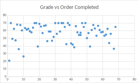
2 Exam 1 grades
Here is a scatterplot showing the lack of correlation between the order in which a student finished exam 1 and the grade.
3 Matlab review
This is my opinion of Matlab.
- Advantages
- Excellent quality numerical routines.
- Free at RPI.
- Many toolkits available.
- Uses parallel computers and GPUs.
- Interactive - you type commands and immediately see results.
- No need to compile programs.
- Disadvantages
- Very expensive outside RPI.
- Once you start using Matlab, you can't easily move away when their prices rise.
- You must force your data structures to look like arrays.
- Long programs must still be developed offline.
- Hard to write in Matlab's style.
- Programs are hard to read.
- Alternatives
- Free clones like Octave are not very good
- The excellent math routines in Matlab are also available free in C++ librarues
- With C++ libraries using template metaprogramming, your code looks like Matlab.
- They compile slowly.
- Error messages are inscrutable.
- Executables run very quickly.
4 Matlab ctd
Finish the examples from last Thurs.
5 Chapter 4 ctd
- Exponential r.v. page 166.
- Memoryless.
- $f(x) = \lambda e^{-\lambda x}$ if $x\ge0$, 0 otherwise.
- Example: time for a radioactive atom to decay.
- Gaussian r.v.
- $$f(x) = \frac{1}{\sqrt{2\pi} \cdot \sigma} e^{\frac{-(x-\mu)^2}{2\sigma^2}}$$
- cdf often called $\Psi(x)$
- cdf complement:
- $$Q(x)=1-\Psi(x) = \int_x^\infty \frac{1}{\sqrt{2\pi} \cdot \sigma} e^{\frac{-(t-\mu)^2}{2\sigma^2}} dt$$
- E.g., if $\mu=500, \sigma=100$,
- P[x>400]=0.66
- P[x>500]=0.5
- P[x>600]=0.16
- P[x>700]=0.02
- P[x>800]=0.001
- Skip the other distributions (for now?).
- Example 4.22 page 169.
- Example 4.24 page 172.
- Functions of a r.v.: Example 4.29 page 175.
- Linear function: Example 4.31 on page 176.
- Markov and Chebyshev inequalities.
- Your web server averages 10 hits/second.
- It will crash if it gets 20 hits.
- By the Markov inequality, that has a probability at most 0.5.
- That is way way too conservative, but it makes no assumptions about the distribution of hits.
- For the Chebyshev inequality, assume that the variance is 10.
- It gives the probability of crashing at under 0.1. That is tighter.
- Assuming the distribution is Poisson with a=10, use Matlab 1-cdf('Poisson',20,10). That gives 0.0016.
- The more we assume, the better the answer we can compute.
- However, our assumptions had better be correct.
- (Editorial): In the real world, and especially economics, the assumptions are, in fact, often false. However, the models still usually work (at least, we can't prove they don't work). Until they stop working, e.g., https://en.wikipedia.org/wiki/Long-Term_Capital_Management . Jamie Dimon, head of JP Morgan, has observed that the market swings more widely than is statistically reasonable.
- Section 4.7, page 184, Transform methods: characteristic function.
- The characteristic function \(\Phi_X(\omega)\) of a pdf f(x) is like its Fourier transform.
- One application is that the moments of f can be computed from the derivatives of \(\Phi\).
- We will compute the characteristic functions of the uniform and exponential distributions.
- The table of p 164-5 lists a lot of characteristic functions.
- For discrete nonnegative r.v., the moment generating function is more useful.
- It's like the Laplace transform.
- The pmf and moments can be computed from it.