This note is under construction.

In Computer Graphics, when you need a curve with increased complexity, the obvious solution is to use a high degree polynomial. That is almost always the wrong answer. This note will give some reasons.

For simplicity, we will use explicit polynomials in 2D, that is, {$ y=f(x) = \sum_{i=0}^{n-1} a_i x^i $}

Consider the common problem of fitting a curve to {$n$} points {$ \{(x_i,y_i) \} $}.

You could use a cubic spline, however, let's fit an exact {$(n-1)$} degree polynomial to those {$n$} points. What could possibly go wrong?

Our test points will be a step function, all the points equally spaced in {$x$}. Half the points will be at {$y=0$}, the rest at {$y=1$}.

{$$x_i = i, 1\le i\le n $$}

{$$y_i = \left\{ \begin{array}{cc} 0 & \mbox{if } 1\le i\le \frac{n}{2} \\ 1 & \mbox{if} \frac{n}{2} < i \le n \end{array} \right. $$}

The process to fit a (n-1) degree polynomial to n points is called Lagrangian interpolation. In Matlab, the polyfit function does it. Here's my code:

 % Plot a Lagrange interpolation to a step function.
 function lagrange2(N);
 n=N/2;
 xp=1:(2*n);
 yp=[zeros(1,n) ones(1,n)];
 p=polyfit(xp,yp,2*n-1);
 x= 0.9 :.1: 2*n+0.1;
 y=polyval(p,x);
 plot(xp,yp,'o:',x,y,'-');

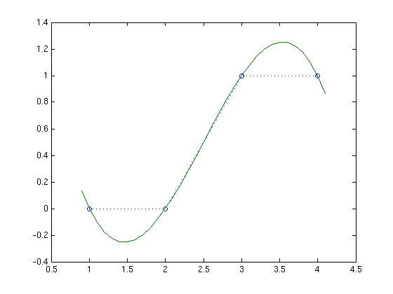
Let's see what this curve looks like. With 4 points, it's good:

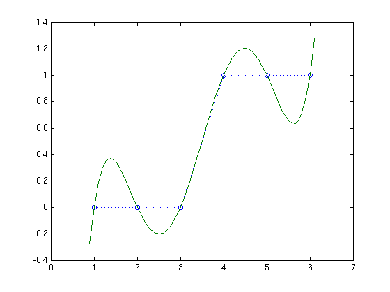
Six points are fine:

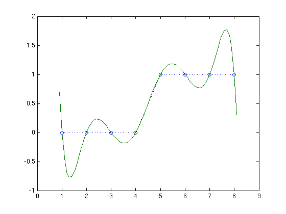
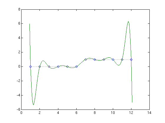
{$n=8$} is still ok, but there's a troubling swing of the curve between the outer two points on each side:

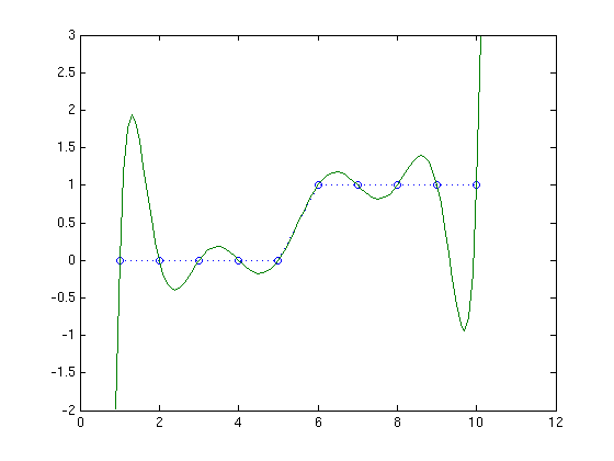
With {$n=10$}, this got worse. The swing is now almost twice as high as the step.

With {$n=12$}, the height of the curve doubled compared to with {$n=10$}. Although the given points have {$ 0\le y\le 1$}, the polynomial has {$y$} up to {$\pm6$}. Also, Matlab is complaining: Warning: Polynomial is badly conditioned. We'll see what that means later.

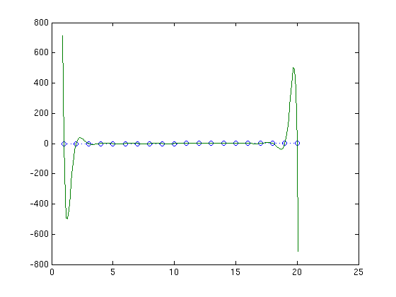
Clearly fitting a single polynomial to many points isn't working. Let's try one final example, {$n=20$} and find the exact 19-th degree interpolating polynomial. Wow! The polynomial ranges up to {$y=\pm 500$}.

Now, let's try moving one point in the middle from {$y=0$} to {$y=1$}. That old and new curves are plotted together.

xxx figure to be inserted xxxxx

The whole curve changed. That's really bad. There's no local control, and it's not even obvious how we got from the points to the curve.

Next, how can we compute the Lagrange? Here is its equation:

{$$ y=f(x) = \sum_{i=1}^n c_i(x) y_i $$}

where

{$$ c_i(x) = \prod_{\substack{j=1\\j\ne i}}^n \frac{x-x_j}{x_i-x_j} $$}

Note that {$ c_i(x_j) = \delta_{ij} $}.

I.e., we can compute coefficients that depend only on the {$x$}'s and then plug on our {$y_i$}. That's nice.

Finally, what's this bad conditioning that Matlab complained about? Let's compute the polynomial coefficients in

{$$ y = f(x) = \sum_{i=0}^{n-1} a_i x^i $$}.

{$$ y_j = \sum_{i=0}^{n-1} a_i {x_j}^i $$}.

{$$ \begin{bmatrix} y_1 \\ y_2 \\ \vdots \\ y_n \end{bmatrix} = \begin{bmatrix} {x_1}^0 & {x_1}^1 & \cdots & {x_1}^{n-1}
{x_2}^0 & {x_2}^1 & \cdots & {x_2}^{n-1}
\vdots & \vdots & \ddots & \vdots
{x_n}^0 & {x_n}^1 & \cdots & {x_n}^{n-1}
\end{bmatrix} \begin{bmatrix} a_0 \\ a_1 \\ \vdots \\ a_{n-1} \end{bmatrix} = M \begin{bmatrix} a_0 \\ a_1 \\ \vdots \\ a_{n-1} \end{bmatrix} $$}

where matrix {$M$} has the powers of the {$x_i$}. It's called a Vandermonde matrix; see Wikipedia:Vandermonde. The problem is that computing the {$a_i$} requires inverting {$M$}, but it is badly conditioned. The larger {$n$} is, the worse the problem is. A lot of significant digits are lost, and there might even be a divide-by-zero during the inversion. You can help by using double precision (almost always you should use double precision), but it's still not a good situation. Even if there isn't an obvious error like the divide-by-zero, the answer will have fewer and fewer correct digits.

(I might add more details later.)

More information is at Wikipedia:Lagrange_polynomial. Finally, Lagrange interpolation was discovered by someone else before Lagrange did. There's the proverb that a discovery is named after the last person to discover it.