PROB Engineering Probability Class 6 Mon 2022-01-31
1 TA office hours
On their webex meeting places.
Hao Lu, luh6@, 2pm Tues
Hanjing Wang, wangh36@, 3pm Fri
If no one has joined in 15 minutes, they will leave.
Write them for other meeting times.
2 Midterm exam 1
Will be in class on Feb 24 or 28. Which do you prefer?
Update: you preferred Feb 28.
3 Leon Garcia, chapter 2, ctd
This is a summary of some of what I presented last week.
-
2.4 Conditional probability, page 47.
big topic
E.g., if it snows today, is it more likely to snow tomorrow? next week? in 6 months?
E.g., what is the probability of the stock market rising tomorrow given that (it went up today, the deficit went down, an oil pipeline was blown up, ...)?
What's the probability that a CF bulb is alive after 1000 hours given that I bought it at Walmart?
definition \(P[A|B] = \frac{P[A\cap B]}{P[B]}\)
-
E.g., if DARPA had been allowed to run its https://en.wikipedia.org/wiki/Policy_Analysis_Market, CNN: Amid furor, Pentagon kills terrorism futures market would the future probability of fictional King Zog I being assassinated be dependent on the amount of money bet on that assassination occurring?
Is that good or bad?
Would knowing that the real Zog survived over 55 assassination attempts change the probability of a future assassination?
-
Consider a fictional university that has both undergrads and grads. It also has both Engineers and others:
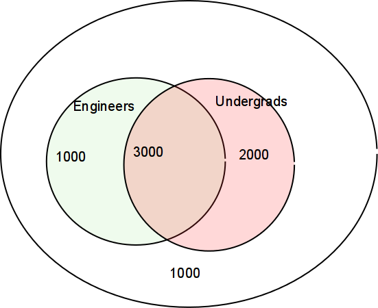
Compute P[E|U], P[E|U'], P[U|E], etc.
\(P[A\cap B] = P[A|B]P[B] = P[B|A]P[A]\)
Example 2.26 Binary communication. Source transmits 0 with probability (1-p) and 1 with probability p. Receiver errs with probability e. What are probabilities of 4 events?
-
Total probability theorem
\(B_i\) mutually exclusive events whose union is S
P[A] = P[A \(\cap B_1\) + P[A \(\cap B_2\) + ...
\(P[A] = P[A|B_1]P[B_1]\) \(+ P[A|B_2]P[B_2] + ...\)
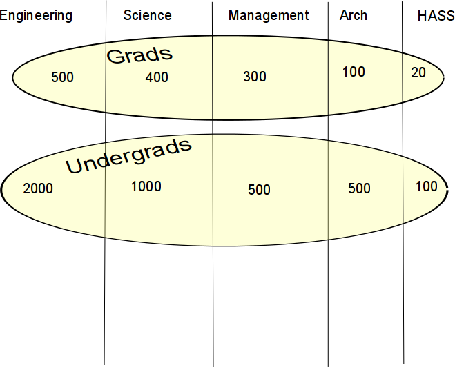
What's the probability that a student is an undergrad, given ... (Numbers are fictitious.)
-
Example 2.28. Chip quality control.
Each chip is either good or bad.
P[good]=(1-p), P[bad]=p.
If the chip is good: P[still alive at t] = \(e^{-at}\)
If the chip is bad: P[still alive at t] = \(e^{-1000at}\)
What's the probability that a random chip is still alive at t?
-
2.4.1, p52. Bayes' rule. This lets you invert the conditional probabilities.
-
\(B_j\) partition S. That means that
If \(i\ne j\) then \(B_i\cap B_j=\emptyset\) and
\(\bigcup_i B_i = S\)
\(P[B_j|A] = \frac{B_j\cap A}{P[A]}\) \(= \frac{P[A|B_j] P[B_j]}{\sum_k P[A|B_k] P[B_k]}\)
-
application:
We have a priori probs \(P[B_j]\)
Event A occurs. Knowing that A has happened gives us info that changes the probs.
Compute a posteriori probs \(P[B_j|A]\)
-
In the above diagram, what's the probability that an undergrad is an engineer?
Example 2.29 comm channel: If receiver sees 1, which input was more probable? (You hope the answer is 1.)
Example 2.30 chip quality control: For example 2.28, how long do we have to burn in chips so that the survivors have a 99% probability of being good? p=0.1, a=1/20000.
-
Example: False positives in a medical test
T = test for disease was positive; T' = .. negative
D = you have disease; D' = .. don't ..
P[T|D] = .99, P[T' | D'] = .95, P[D] = 0.001
P[D' | T] (false positive) = 0.98 !!!
-
Multinomial probability law
There are M different possible outcomes from an experiment, e.g., faces of a die showing.
Probability of particular outcome: \(p_i\)
Now run the experiment n times.
-
Probability that i-th outcome occurred \(k_i\) times, \(\sum_{i=1}^M k_i = n\)
\begin{equation*} P[(k_1,k_2,...,k_M)] = \frac{n!}{k_1! k_2! ... k_M!} p_1^{k_1} p_2^{k_2}...p_M^{k_M} \end{equation*}
Example 2.41 p63 dartboard.
Example 2.42 p63 random phone numbers.
-
2.7 Computer generation of random numbers
Skip this section, except for following points.
Executive summary: it's surprisingly hard to generate good random numbers. Commercial SW has been known to get this wrong. By now, they've gotten it right (I hope), so just call a subroutine.
The Mersenne Twister is a common hi-quality RNG.
Arizona lottery got it wrong in 1998.
Even random electronic noise is hard to use properly. The best selling 1955 book A Million Random Digits with 100,000 Normal Deviates had trouble generating random numbers this way. Asymmetries crept into their circuits perhaps because of component drift. For a laugh, read the reviews.
Pseudo-random number generator: The subroutine returns numbers according to some algorithm (e.g., it doesn't use cosmic rays), but for your purposes, they're random.
Computer random number routines usually return the same sequence of number each time you run your program, so you can reproduce your results.
You can override this by seeding the generator with a genuine random number from linux /dev/random.
2.8 and 2.9 p70 Fine points: Skip.
-
Review Bayes theorem, since it is important. Here is a fictitious (because none of these probilities have any justification) SETI example.
A priori probability of extraterrestrial life = P[L] = \(10^{-8}\).
For ease of typing, let L' be the complement of L.
Run a SETI experiment. R (for Radio) is the event that it has a positive result.
P[R|L] = \(10^{-5}\), P[R|L'] = \(10^{-10}\).
What is P[L|R] ?
-
Some specific probability laws
In all of these, successive events are independent of each other.
A Bernoulli trial is one toss of a coin where p is probability of head.
We saw binomial and multinomial probilities in class 4.
The binomial law gives the probability of exactly k heads in n tosses of an unfair coin.
The multinomial law gives the probability of exactly ki occurrances of the i-th face in n tosses of a die.
4 Bayes theorem ctd
-
We'll do the examples.
We'll (re)do these examples from Leon-Garcia in class.
-
Example 2.28, page 51. I'll use e=0.1.
Variant: Assume that P[A0]=.9. Redo the example.
Example 2.30, page 53, chip quality control: For example 2.28, how long do we have to burn in chips so that the survivors have a 99% probability of being good? p=0.1, a=1/20000.
-
Event A is that a random person has a lycanthopy gene. Assume P(A) = .01.
Genes-R-Us has a DNA test for this. B is the event of a positive test. There are false positives and false negatives each w.p. (with probability) 0.1. That is, P(B|A') = P(B' | A) = 0.1
What's P(A')?
What's P(A and B)?
What's P(A' and B)?
What's P(B)?
You test positive. What's the probability you're really positive, P(A|B)?
5 Chapter 2 ctd: Independent events
-
2.5 Independent events
\(P[A\cap B] = P[A] P[B]\)
P[A|B] = P[A], P[B|A] = P[B]
A,B independent means that knowing A doesn't help you with B.
Mutually exclusive events w.p.>0 must be dependent.
-
Example 2.33, page 56.
-
More that 2 events:
N events are independent iff the occurrence of no combo of the events affects another event.
Each pair is independent.
Also need \(P[A\cap B\cap C] = P[A] P[B] P[C]\)
This is not intuitive A, B, and C might be pairwise independent, but, as a group of 3, are dependent.
See example 2.32, page 55. A: x>1/2. B: y>1/2. C: x>y
Common application: independence of experiments in a sequence.
-
Example 2.34: coin tosses are assumed to be independent of each other.
P[HHT] = P[1st coin is H] P[2nd is H] P[3rd is T].
-
Example 2.35, page 58. System reliability
Controller and 3 peripherals.
System is up iff controller and at least 2 peripherals are up.
Add a 2nd controller.
2.6 p59 Sequential experiments: maybe independent
-
2.6.1 Sequences of independent experiments
Example 2.36
-
2.6.2 Binomial probability
Bernoulli trial flip a possibly unfair coin once. p is probability of head.
(Bernoulli did stats, econ, physics, ... in 18th century.)
-
Example 2.37
P[TTH] = \((1-p)^2 p\)
P[1 head] = \(3 (1-p)^2 p\)
Probability of exactly k successes = \(p_n(k) = {n \choose k} p^k (1-p)^{n-k}\)
\(\sum_{k=0}^n p_n(k) = 1\)
Example 2.38
Can avoid computing n! by computing \(p_n(k)\) recursively, or by using approximation. Also, in C++, using double instead of float helps. (Almost always you should use double instead of float. It's the same speed.)
Example 2.39
Example 2.40 Error correction coding
6 Bayes theorem ctd
-
We'll do the defective item example, using both numbers and Bayes rule.
We'll redo these examples from Leon-Garcia in class.
Example 2.28, page 51. Assume P[A0]=1/3. P[e]=.1 What is P[A0|B0]?
Example 2.30, page 53, chip quality control: For example 2.28, how long do we have to burn in chips so that the survivors have a 99% probability of being good? p=0.1, a=1/20000.
-
3.3.2 page 109 Variance of an r.v.
That means, how wide is its distribution?
Example: compare the performance of stocks vs bonds from year to year. The expected values (means) of the returns may not be so different. (This is debated and depends, e.g., on what period you look at). However, stocks' returns have a much larger variance than bonds.
\(\sigma^2_X = VAR[X] = E[(X-m_X)^2] = \sum (x-m_x)^2 p_X(x)\)
standard deviation \(\sigma_X = \sqrt{VAR[X]}\)
\(VAR[X] = E[X^2] - m_X^2\)
2nd moment: \(E[X^2]\)
also 3rd, 4th... moments, like a Taylor series for probability
shifting the distribution: VAR[X+c] = VAR[X]
scaling: \(VAR[cX] = c^2 VAR[X]\)
Derive variance for Bernoulli.
-
Example 3.20 3 coin tosses
general rule for binomial: VAR[X]=npq
Derive it.
Note that it sums since the events are independent.
Note that variance/mean shrinks as n grows.
Geometric distribution: review mean and variance.
-
Suppose that you have just sold your internet startup for $10M. You have retired and now you are trying to climb Mt Everest. You intend to keep trying until you make it. Assume that:
Each attempt has a 1/3 chance of success.
The attempts are independent; failure on one does not affect future attempts.
Each attempt costs $70K.
Review: What is your expected cost of a successful climb?
$70K.
$140K.
$210K.
$280K.
$700K.
3.4 page 111 Conditional pmf
-
Example 3.24 Residual waiting time
X, time to xmit message, is uniform in 1...L.
If X is over m, what's probability that remaining time is j?
\(p_X(m+j|X>m) = \frac{P[X =m+j]}{P[X>m]} = \frac{1/L}{(L-m)/L} = 1/(L-m)\)
\(p_X(x) = \sum p_X(x|B_i) P[B_i]\)
-
Example 3.25 p 113 device lifetimes
2 classes of devices, geometric lifetimes.
Type 1, probability \(\alpha\), parameter r. Type 2 parameter s.
What's pmf of the total set of devices?
Example 3.26, p114.
3.5 p115 More important discrete r.v
Table 3.1: We haven't seen \(G_X(z)\) yet.
-
3.5.1 p 117 The Bernoulli Random Variable
We'll do mean and variance.
Example 3.28 p119 Variance of a Binomial Random Variable
Example 3.29 Redundant Systems
-
3.5.3 p119 The Geometric Random Variable
It models the time between two consecutive occurrences in a sequence of independent random events. E.g., the length of a run of white bits in a scanned image (if the bits are independent).
-
3.5.4 Poisson r.v.
The experiment is observing how many of a large number of rare events happen in, say, 1 minute.
E.g., how many cosmic particles hit your DRAM, how many people call to call center.
The individual events are independent. (In the real world this might be false. If a black hole occurs, you're going to get a lot of cosmic particles. If the ATM network crashes, there will be a lot of calls.)
The r.v. is the number that happen in that period.
-
There is one parameter, \(\alpha\). Often this is called \(\lambda\).
\begin{equation*} p(k) = \frac{\alpha^k}{k!}e^{-\alpha} \end{equation*} Mean and std dev are both \(\alpha\).
In the real world, events might be dependent.
Example 3.32 p123 Errors in Optical Transmission
3.5.5 p124 The Uniform Random Variable