Summary

Local topological data structures, uniform grids, KISS lead to fast implementations on large datasets.

Example: Mass Props

• 100,000,000 squares (400,000,000 edges)...
• edge length = 0.0006
• Average depth of squares = 37
• Number of potential edge-edge intersections = 15,000,000,000
• Time to find area, perimeter of union: 640 cpu secs.

(500 squares illustrated.)

Application: Cutting Tool Path

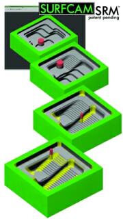
• Represent path of a tool as piecewise line.
• Each piece sweeps a polyhedron.
• Volume of material removed is (approx) volume of union of those polyhedra.

(Image shows Surfware Inc's Surfcam.)

More Applications

VLSI Design

Sometimes polygons are designed as overlapping squares.

Cartographic Regions

Existing Method for Union Area

• Unite the input polygons pair by pair, using DCELs, quad-edges, or whatever.
• Repeat log(N)=23 times, forming larger polygons.
• Carefully watch the topology and the intermediate storage swell.
• Compute the area and perimeter.

Problems With Usual Method for Area of Union of Many Objects

• 
• Large depth of squares is bad (more intersections, slower inclusion testing).

New Technique

Principles

• Keep the data structures as simple and compact as possible.
• Store the minimal possible topology.

Specifics

• Few pointers
• No hierarchies
• No global topology. Not even edges.

Output Polygon Format

Only data type is vertex, containing

• (x,y)
• directions of its edges
• which sector is inside

Properties

• no explicit edges; no edge loops
• no component containment info
• can represent general polygons with multiple nested or separate components
• any mass property determinable in one pass thru the set
• parallelizable
• amenable to external storage implementation

Mass Properties of Rectilinear Polygons

• 8 types of vertices, based on neighborhood
• 4 are type "+", 4 "-"
• Area = (s_ix_iy_i)
• Perimeter = (+-x_i+-y_i)

Formulae generalize to other polygons, and to 3D.

Finding the Output Vertices

An output vertex is either:

• Input vertex, or
• Intersection of two edges

but only some of them (10^-6 in the big example).

specifically those vertices and intersections that are not inside any other square.

Required Operations

• Edge intersection
• Point inclusion

Edge intersection

• Optimize for many small edges.
• Do only rectilinear edges here (easier; no roundoff)
• N = number of edges
• L = edge length (fraction of universe)
• M = expected number of intersections = (NL/2)²

Time = N*log(M) is too slow.

Even linear time is too slow.

Even linear time is too slow?!

The expected number of intersections is (NL/2)²

but

The expected number of intersections that become output vertices is O(N).

regardless of the depth complexity.

Why? The graph of output vertices, edges is planar.

Edge Intersection by Uniform Grid

• Superimpose a grid on the data.
• Typical cell size = 1/3 edge length.
• For each edge, find which cells it passes thru.
• Then, for each cell, compare its edges pairwise for intersection.

Properties

• Expected time = size(input) + size(output)
• Parallelizable
• Does red-blue intersection well
• Can be destroyed by adversarial input, but never been seen in practice.
• Flat works. Not necessary to refine hierarchically in denser regions.

Aside: Red-Blue Intersection

• Application: does this red object intersect this blue one?
• Given: N red edge segments, and N blue ones.
• There may be O(N²) red-red and blue-blue intersections.
• You don't know them.
• There are O(1) red-blue intersections.
• Find them.
• No subquadratic worst-case algorithm (SFAIK).

Moral: sometimes heuristics are necessary.

Time Details

(N edges, len L, cell size C)

• Num (cell, edge) pairs: N(L/C+1)
• Ave num edges/cell: NC(L+C)
• Expected number of intersections = M = O(N²L²)
• Total work intersecting edges in cells: N²(L+C)²
• Total cost: N(L/C+1)+ N²(L+C)²
• If C=cL, cost = N+N²L
  = N + M

Other Edge Intersection by Uniform Grid Examples

Varying edge lengths are not a problem.

Uniform Grid and Covering Squares

• Only visible intersections contribute to the output.
• That's often a small fraction - inefficient.
• In the big example (100,000,000 squares, len 0.0006), 15,000,000,000 total intersections, but only 13,109 visible.
• Solution: add the squares themselves to the grid.

Solution: add the squares themselves to the grid.

• For each square, find which cells it completely covers.
• (Edges were different.)
• If a cell is completely covered by a square, then nothing in that square can contribute to the output.
• Delete all edges from covered squares.
• Some edges may also be incident on noncovered squares. Keep that info.
• Intersect pairs of edges in the noncovered squares.

If the cell size is somewhat smaller than the edge size then almost all the hidden intersections are never found. Good.

Expected time = size(input) + size(useful intersections).

Point Containment Testing

Q: How to test if a point P is contained in at least one square?

A: Start with the Jordan curve method. (Run a ray from P to infinity.)

Optimizations:

- Since the edges are oriented, sufficient to stop at the first edge.

Optimizations ctd

• If no edge is in this cell, then the whole cell is covered, and we would not be testing P.
• Test P against every edge in its cell, to see if any edge belongs to a square containing P.
• Since cells are made smaller than squares, two opposite edges of the same square are not both in the cell, so the test gets a little simpler.

Time per point: proportional to average number of edges per cell. Constant (for certain cell sizes).

SoS for Degeneracies

Many degeneracies.

Use SoS.

If 2 coordinates compare equal, then compare on the edge number.

Determining Intersection Neighborhoods

Intersection Neighborhoods needed for area computation.

We know the 2 edges creating the intersection, including the edges' orientation.

That's enough.

Extension to General Polygons

The only data type is the incidence of an edge and a vertex, and its neighborhood. For each such:

• V = coord of vertex
• T = unit tangent vector along the edge
• N = unit vector normal to T pointing into the polygon.

Polygon: {(V, T, N)} (2 tuples per vertex)

Perimeter = -sum(V.T).             Area = 1/2 sum( V.T V.N )
Multiple nested components ok.

Extension to 3D

The only data type is the incidence of a face, an edge and a vertex, and its neighborhood. For each such:

• V = coord of vertex
• T = unit tangent vector along the edge
• N = unit vector normal to T in the plane of the face, pointing into the face.
• B = unit vector normal to T and N, pointing into the polyhedron.

Polyhedron: {(V, T, N, B)}

Perimeter = -1/2 sum(V.T)           Area = 1/2 sum( V.T V.N )
Volume = -1/6 sum( V.T V.N V.B )

Implementation Validation

• The expected area is 1-(1-L²)^S, if S = number of squares.
• Compare to computed area.
• Assume that coincidental equivalence is unlikely.

  Data Validity Test

  These formulae require consistent data.

  Use that to validate the input data:

  • Randomly rigidly transform the polyhedron
  • If the computed mass properties change, the data is inconsistent.
  • Otherwise, repeat.
  
  

  Volume, Area, Edge Length of Union of Cubes

  
  • (proposed)
  • Use a 3D uniform grid.
  • Check for cubes completely covering grid cells.
  • Insert edges, faces.
  • Determine edge-face intersections.
  • No big changes, just messier.

  100,000,000 Squares: Implementation

  • Environment: 1600 MHz Pentium, 768 MB memory, Linux SuSE 8.0, gcc 2.95
  • 979 lines (25KB) of code including comments. Executable code size = 24KB.
  • Elapsed time to implement: 2 weeks, but based on earlier programs and thinking going back to 1970s.

  100,000,000 Squares: Times

  • CPU time to make squares and put into cells = 112 secs
  • to put edges into cells = 300 secs
  • to process vertices and intersections in cells = 229 secs
  • TOTAL = 640 secs

  This could probably be hand optimized.

  100,000,000 Squares: Storage

  • 4 bytes per square (16 bit coords: x0, y0).
  • 8 bytes per grid cell: # alloc edges, # actual edges, pointer to edge array.
  • 4+ bytes (cell,edge): edge number. (Allocated in batches with spares).

  Could use external storage. E.g., Write (cell,edge) as found.

  
  

  100,000,000 Squares: Numbers

  • # squares = 100,000,000
  • # edges = 400,000,000           Edge length = 0.0006
  • Average depth of squares = 37
  • Grid: 4000x4000
  • # Edge-cell insertions = 1,376,574,038
  • # Edge-cell pairs deleted from covered cells = 1,376,039,891
  • # Cells completely covered by squares = 15,983,949
  • Predicted # edge-edge intersections = 15,000,000,000
  • # intersections found = 1,495,245
  • # visible intersections = 13,109
  
  

  Related Implementation: Connected Components

  
  • Connected components of a 1024*1088*1088 universe with 1,212,153,856 1-bit voxels.
    Typical time to find the 4,539,562 components: 96 seconds.
  • For a 2-D example with 18573*19110=354,930,030 1-bit pixels, CPU time to find 32858 components: 25 secs.
  
  

  Related Implementations: Map Overlay Areas

  

  Area of non-empty intersections of the polygons in 2 planar maps: E.g. overlay counties of the coterminous US against hydrography polygons. Map stats:

  Map #0: 55068 vertices, 46116 edges, 2985 polygons
  Map #1: 76215 vertices, 69835 edges, 2075 polygons
  

  Total time (excluding I/O): 1.58 CPU seconds.

  
  

  Summary

  Local topological data structures, uniform grids, KISS lead to fast implementations on large datasets.

  

  ---

  Dr. Wm Randolph Franklin,
  Email: wrfATecse.rpi.edu
  http://wrfranklin.org/
  ☎ +1 (518) 276-6077; Fax: 6261
  ECSE Dept., 6026 JEC, Rensselaer Polytechnic Inst, Troy NY, 12180 USA
  (GPG and PGP keys available)
  

  ---

  Copyright © 1994-2002, Wm. Randolph Franklin. You may use my material for non-profit research and education, provided that you credit me, and link back to my home page.