Terrain Elevation Data Structure Operations
Wm Randolph Franklin
Michael B Gousie
Goal
-
Operate on terrain elevation data.
-
Compare competing representations on large datasets
-
Integrate into a system
Operations:
-
Visibility
-
Compression
-
Interpolate contours to grid
-
Approx grid to TIN
-
Drainage (future)
How the Parts Fit Together
Theme
-
Experimental Computational Cartography
-
Interface between the theoreticians and the computer
-
Design then implement algorithms and data structures
-
efficiently
-
on the largest (not toy sized!) datasets
-
then
-
observe results and
-
suggest new research problems
-
use general purpose data structures and algorithms,
-
benefit from larger community effort
-
like using Open Source Software instead of proprietary packages.
-
Notable special-purpose failures: Lisp machines, floating point processors,
database engines, special graphics engines, and most parallel machines.
What's New?
... since people have converted data for several decades
now.
-
hardware,
-
SW packages,
-
specific algorithms.
Historical Context
-
Various formats possible for Hypsographic (elevation) data
-
Triangulated Irregular Networks (TINs),
-
grids or arrays, and
-
contour lines.
-
Which is best?
-
Criteria:
-
complexity, size, and accuracy
-
need for conversion algorithms.
-
need for a measure of goodness for approx conversions.
-
simplest: RMS error.
-
more useful: effect on
-
visibility, drainage, slope
Research Program Components
-
Conversion from DEM to TIN
-
Visibility
-
DEM Compression
-
Interpolating from Contours to DEM
Conversion from DEM to TIN
-
I designed possibly the first TIN program in GIS, in 1973.
-
Now, can easily completely TIN a complete 1201x1201 DEM.
Example - Lake Champlain West DEM
-
1201x1201
-
Can process to over 1,000,000 triangles.
-
However, max error < 1 after 600,000 triangles.
-
Here is original, then after 1024, 2048, 4096, 8192, 16384, 32768, 65536
points inserted.
Extensions:
-
How does error correlate to number of triangles?
-
Is a Delauney triangulation the best?
-
Is a constrained triangulation, forcing features to be included, necessary?
-
Should we alternate inserting and deleting points?
Visibility
-
viewshed: What points can an observer see?
-
Visibility indices: How much area can each
possible observer see?
Extensions:
-
Compute confidence intervals.
-
Unshaded (
 ): almost certainly visible.
-
Lightly shaded (
 ): probably visible.
-
Darkly shaded (
 ): probably hidden.
-
Black (
 ): almost certainly hidden.
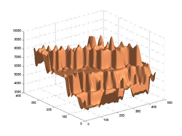
Sample viewshed output
Following are two images:
-
some sample terrain from South Korea, color-coded by elevation, and
-
the visibility indices of every point, colored similarly.
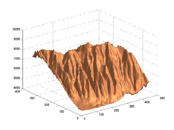
Sample Terrain; Visibility Indices
Extensions:
-
siting observers: alternate the above 2 programs.
-
feature determination
-
small relation of height to visibility
Siting Observers
Programs viewshed and vix may be used to find
a set of observers that jointly can see every point as follows.
-
Use vix to list all the points by visibility index, and hence,
to find the most visible point. Place the first observer, O1,
there.
-
Use viewshed to find the points that O1 cannot see.
-
Filter the sorted list of points to delete points that O1 can
see.
-
Find the most visible point that O1 cannot see; that is the
second observer, O2.
-
Repeat until the set of observers can see every point.
DEM Compression
-
Hypothesis: The
effort spent on image compression might transfer to elevations.
-
Differences: one
channel, 16 bits, different measure of goodness
-
Uses: Said and Pearlman's
wavelet program
-
Test cases: 24 USGS
level-1 1201x1201 DEMs.
-
Today's example: level-2
30-meter DEM of Bountiful Utah.
-
Standard deviation of the elevations: 1096
meters,
-
= RMS error if the file was compressed to two bytes
-
W/o compression: 11 bits per point (bpp).
-
Lossless compression: 5.234 bpp
-
Lossy compression, size vs error:
| BPP |
RMS Error, m |
| 5.234 |
0.0 |
| 1.0 |
6.0 |
| 0.1 |
51.7 |
| 0.03 |
148 |
| 0.01 |
535 |
| 0.0 |
1096 |

Original

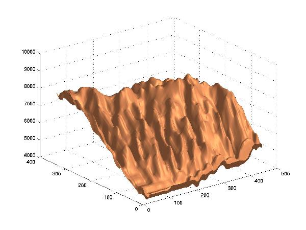
Lossy Compression to 1 Bit/Point, RMSE=6.0 meters
Lossy Compression to 0.1 Bit/Point, RMSE=51.7 m
Lossy Compression to 0.03 Bit/Point, RMSE=148 m
Lossy Compression to 0.01 Bit/Point, RMSE=535
Interpolating from Contours to DEM
Prior Art
-
Interpolate in vertical planes.
-
PDE - Lagrange (heat flow) or thin-plate
-
Extend straight lines out in 8 directions to the
nearest contour
-
Voronoi diagram / Delaunay triangulation, e.g. area
stealing
-
Medial axis
-
Inverse distance weighting.
-
Detect features, interpolate them, then fill in.
Limits of Existing Methods
-
Often tested only on synthetic, small, datasets.
-
May require unbroken contours.
-
May require contours be thinned.
-
Generated triangles may be horizontal, or long & thin.
-
Generated peaks may be flat.
-
May generate terraces and ringing.
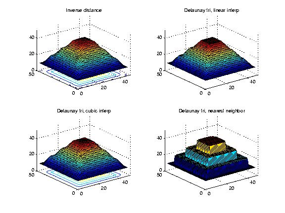
Figure: Interpolating 3 Nested Squares with Inverse Distance
Weighting, and 3 Ways with Delaunay Triangles
Interpolation & Approximation Introduction
Desirable properties:
-
local control
-
variation minimization
-
interpolation
-
conformal
-
Don't want to see the contours in the result.
-
Peak inside top contour and valley outside outer contour.
The math is counterintuitive, and the desired properties mutually contradictory.
Goodness Criteria
Ideal:
-
Maximum likelihood surface fitting the data.
-
Requires: Formal probability model of terrain elevation.
-
which is still incompletely solved. (e.g., long range correlations from
drainage patterns).
Next best:
-
What looks good?
-
Shaded plots
-
Profiles
-
Statistically compare curvature at generated points on/near data points
against farther points. (future)
Partial differential equations (PDEs)
Laplacian, or heat-flow equation,
zxx+zyy = 0,
where
zxx = d2z/dx2
solved by iteration on a grid,
4zij = zi-1,j + zi+1,j + zi,j-1
+ zi,j+1.
Problem: demonstrates the terracing artifact.
The thin plate model minimizes total curvature.
zxx2 + 2zxy2 + zyy2
= 0;
20zij = 8(zi-1,j + zi+1,j + zi,j-1
+ zi,j+1) - 2(zi-1,j-1+zi-1,j+1+zi+1,j-1+zi+1,j+1)
- (zi-2,j + zi+2,j + zi,j-2 + zi,j+2)
Intermediate Contours
Our first new method repeatedly interpolates new contour lines between
the original ones, somewhat similar to the medial axis. If two adjacent
contour lines are: A, at elevation
a, and B, at b,
then we interpolate at elevation (a+b) thus.
-
Pick a point on A.
-
Find the closest point on B (approximating the gradient).
-
The midpoint is on the intermediate contour.
Our contrarian philosophy is that we don't find the elevation at certain
points, but rather find points with a certain elevation.
Figure: Crater Lake: Original Contours and Intermediate Contour
Interpolation
The Maximum Intermediate Contours (MIC) method iterates the process.
Gradient Lines
-
like lofting in CAGD.
-
Calculate gradient lines.
-
Refine their elevations.
Example:
900x900 piece of the Crater Lake DEM.
|
Figure 6. Crater Lake: Original Contours
|

Figure 7. Thin Plate Approx
|
Figure 8. Intermediate Contour Approx
|
Figure 9. Gradient Line Approx
|
Overdetermined Laplacian Solution
-
The problem with many existing methods is that no information flows across
the contours. This causes terracing.
-
Make the known data points also be the average of their neighbors.
-
assume that there are N2 unknowns; i.e., even the known
points are unknown. There are now two types of equations. First, for all
points:
4zij = zi-1,j + zi+1,j + zi,j-1
+ zi,j+1
-
Second, for the known points, we make an equation that they are equal to
their known values:
zij = hij
-
Do a best-fit solution.
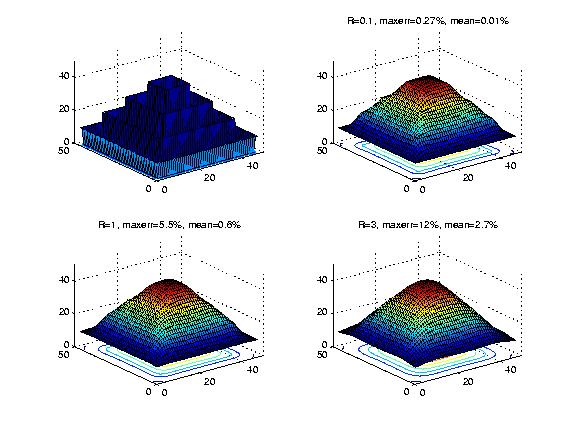
Figure: Overdetermined Laplacian PDE, Weighting Different
Equations Differently
Table: Error versus Weight
| R |
Max % Error |
Mean % Error |
| 0.1 |
0.27 |
0.01 |
| 1.0 |
5.5 |
0.6 |
| 3.0 |
12 |
2.7 |
Proposed Future Work
Short Term
-
Multiple observers covering a region.
-
Fast graphics cards?
-
Test the largest DEM datasets available.
-
Study other serendipitous questions that will arise.
Medium Term
-
Leverage from array operations tools, like Matlab?
-
Output sensitivity to input?
-
If visibility indices and viewsheds are sensitive to small input perturbations,
then
-
Try to establish error bounds on the output.
-
Faster and less accurate output when input is inaccurate?
-
Feature recognition: feed into constrained TIN.
Long Term
-
Investigate the general question of the proper representation of terrain
elevation data.
-
If using TINs, use triangular splines, not just piecewise multilinear flat
triangles.
-
Consider the idea of a conceptually deeper representation, based on the
geomorphological forces that created the terrain. Devise a basis set of
operators, such as uplift, downcut, etc. Deduce the operators
that created the particular terrain under consideration, and store them.
-
Slightly differently, represent the terrain by the features that people
would use to describe it. This idea is many decades old. Can we get it
to work? The problem is that you can't just say that there is a hill
over there, you have to specify the hill in considerable detail,
which would seem to take more space than simply listing all the elevations
with a grid or TIN.
-
Extend to geological data structures. Plan excavation strategy for open
pit mine.
-
The major creative force for terrestrial terrain is water erosion.
This does not apply to the moon, Venus, and, to the same extent, to Mars.
Therefore those surfaces might be statistically different. What impact,
if any, would this have on the speed and output distribution of our algorithms
and data structures?
How the Parts Fit Together