): almost certainly visible.
 ): probably visible.
 ): probably hidden.
 ): almost certainly hidden.
We describe several programs working with 1201x1201 gridded (array) terrain elevation data: determining the viewshed of an observer, and the visibility indices of all points, converting from a grid to a TIN, losslessly and lossily compressing a grid, and interpolating from contours to a grid. The intent is to integrate these, and new, programs, into a test suite the better to understand hypsography.
Keywords: contours, interpolation, grids, elevation, visibility, compression, triangulated irregular network
Hypsographic (elevation) data can be represented in various formats, including Triangulated Irregular Networks (TINs), grids or arrays, and contour lines. The various formats compete on factors such as complexity, size, and accuracy; it is not clear which will eventually dominate. Since data may often be available in only one format, there is a need for conversion algorithms. Since a conversion is generally only approximate, there is a need for a measure of goodness. Altho the simplest criterion is the root-mean-square (RMS) error of the approximation, more sophisticated criteria, such as the effect on important cartographic properties such as visibility and drainage would be more useful.
Many (but not all) of the techniques described here are based upon classic ideas, known for decades. However, useful new techniques and packages from Mathematics and Computer Science are now available, such as multigrids and Matlab. This makes old ideas, such as directly solving a heat-flow (Laplacian) partial differential equation on a large grid, feasible for the first time. Also, larger datasets raise new special cases. Finally, faster and larger hardware allows new implementation techniques, e.g., a program with arrays of 10,000,000 elements is now routine.
We try to use general purpose data structures and algorithms, which are attractive because they have benefitted from the larger community effort devoted to improving them. This is analogous to the argument for using Open Source Software instead of proprietary packages. Notable commerical failures of special-purpose HW and SW include: Lisp machines, floating point processors, database engines, special graphics engines, and most parallel machines. Finally, careful algorithm implementation helps to keep the code small and fast.
This web page is an expanded version of a talk presented in August 1999 at ICA1999 - The 19th International Cartographic Conference & The 11th General Assembly of ICA
The following sections will describe the various components of our terrain elevation research program.
Various programs for extracting a Triangulated Irregular Network from a set of elevation points exist (altho some have been demonstrated only on toy datasets); perhaps the first was Franklin (1973). A regular grid of data is somewhat harder to process than a random array of points because of various degeneracies such as the most deviant point in a triangle being on an edge, causing one of the three new triangles to degenerate to a line segment. Our program, Franklin (1994), can process a complete, 1201x1201 level-1 DEM, producing 200,000 triangles.
This conversion process also shows the difficulty of predicting the behavior of even a simple idea. One might expect that splitting a triangle into three smaller triangles, at its worst point, reduces the maximum deviation. However, as various researchers have observed, sometimes the maximum deviation doubles. Altho unexpected, this isn't a problem since when the new worst triangle is split, the max deviation drops dramatically.
Consider the elevation of a region of terrain, together with an observer and target(s). Can the observer see the target? What targets can the observer see? Where are the best places for the observer?
We describe some existing programs to answer these questions, and then propose future work. This is based on the PhD work of Ray (1994). For more details, see Franklin & Ray (1994). All these programs are very efficient on large databases.
The terrain universe is defined by a square array of NxN elevations.
The observer is (x,y,h), a point in the terrain, plus a height above the surface, for the usual case that the observer is above the terrain.
The target is also a point in the terrain. Sometimes a height above the surface may be specified. At other times, the programs report the minimum height above the surface at which a target over that point becomes visible by the specified observer.
Program viewshed finds the viewshed, or visibility polygon, or the set of points in the terrain that can be seen by a given observer who may be a specified height above the surface. Although a viewshed is defined only for some target height, viewshed also computes the minimum visible elevation, or the lowest height at the point that is visible by the observer, of every point in the terrain.
Viewshed operates by working out from the observer in square rings. The iteration invariant, which is known for each point of one ring before the next ring is computed, is the minimum elevation above that point that is visible. If the point is visible, then that minimum is zero.
Note that these minimum visible elevations for a ring encapsulate most of the relevant terrain elevation information for points inside the ring. Once a ring is computed the interior points will not be considered again.
To compute the minimum visible elevation for a target point in the next ring out, a line of sight (LOS) is drawn from the observer to the target point. This LOS will pass between two adjacent points in the adjacent inside ring. The LOS is made to pass between these points at the minimum visible elevation. Then, its elevation at the target becomes the minimum visible elevation of the target.
Since it is impossible for one elevation post to completely represent the elevation throughout a square of terrain, and impossible for two posts to represent the elevation along the whole line segment between them, thru which the LOS is passing, some approximation is required. This can be biased as desired. The LOS may be made to pass between the two adjacent points at an elevation linearly interpolated from its relative distance between them, or at the greater of their two elevations, or at the lesser elevation. The first method (interpolation) is perhaps the most accurate, although it has an subtle uncertainty that grows with the ring size. The second (max) biases the minimum visible elevations on the high side, while the third (min) biases the minimum visible elevations in the low direction.
This means that for a given target elevation, we can classify each point in the terrain thus:
target points that are almost certainly hidden, since the minimum visible elevation calculated with the min approximation is above the target elevation.
target points that are probably hidden since the target elevation is below the interpolated minimum visible elevation.
target points that are probably visible since the target elevation is above the interpolated minimum visible elevation.
target points that are almost certainly visible since the target elevation is above the minimum visible elevation calculated with the max approximation.
Viewshed is extremely fast. On a 75 MHz Pentium, recomputing the viewshed for a 300x300 terrain takes under 0.5 CPU second. Indeed, on some platforms, the visibility computation is faster than the frame buffer updating. The asymptotic execution time is linear in the number of terrain points, which is quite favorable compared to algorithms that theoretically calculate the exact visibility. Also, an exact computation is not justified, given the inexact input. Our philosophy is good enough accuracy.
Below is a sample of viewshed's operating on a 300x300 piece of the Lake Champlain West level-1 USGS DEM. Elevation is indicated by color (or shades of gray), as shown on the scale along the right side. The observer was located at the highest point in the terrain, and about 15 meters above ground level. The target was assumed to be about 15 meters up, the visibility was calculated 3 ways as described above, in about 1 CPU second total on the 75MHz Pentium, and the terrain was shaded accordingly:
): almost certainly visible.
): probably visible.
): probably hidden.
): almost certainly hidden.
Figure 1. Sample viewshed output
The figure shows that the visibility status of over half of the points in this example is actually uncertain. That is quite unexpected. If this uncertainty is intrinsic to the data, rather than an artifact of our approximate algorithm, then we have an important subject for future research.
Vix finds the visibility index, or the area of the viewshed, of every point in the terrain.
We do not find each point's explicit viewshed, but rather use sampling techniques to estimate its area. For each observer, perhaps 32 rays are fired out at equally spaced angles towards the edge of the terrain. Along each ray, a subset of the points are selected, and a one-dimensional line-of-sight algorithm is executed on them, to compute the number of visible points, in time linear in the number of points tested. The visibility index of the observer is the fraction of tested points that are visible.
Vix then repeats this process for all N2 possible observers.
Following are two images:
some sample terrain from South Korea, and
the visibility indices of every point, with bright points being more visible.
|
Figure 2. Sample Terrain |
Figure 3. Visibility Indices |
Some notable points are these:
The north-south ridge in the center is sharpened.
The lowest region is the water at the south near the west, but its visibility indices are surprisingly high.
In contrast, the high mountainous region in the north center is not so visible.
There is often little correlation between elevation and visibility index, as seen in this scatterplot of the above data (whose correlation coefficient is very slightly negative).

Note that our algorithm is performing a classic statistical sampling and estimation. We estimate the fraction of all the points that are visible by testing a subset. Assuming that our sampling is uncorrelated with the points' visibility, computing the standard deviation in our estimate is easy. A check is also possible by dividing the rays alternately into two groups, computing the visibility index separately for each group, and measuring the significance of the difference in the means with a T-test. Vix could be extended to use this adaptively so to fire only the minumum necessary number of rays.
Given the visibility index of each point,determining the identity of the most visible points is trival. In addition, if only their locations is required, less accuracy in the visiblity index computation may be appropriate.
Programs viewshed and vix may be used to find a set of observers that jointly can see every point as follows.
This process can be refined as follows.
When selecting Oi for i>1, instead of choosing the most visible remaining point, test the several most visible remaining points, and choose the one that can see the most remaining points. This corrects for points whose viewsheds largely overlap each other.
(That problem is less serious than one might suppose. Indeed a very visible point tends to dominate its neighbors, so that they are not very visible.)
The programs described here use gridded elevation data. Some others use a Triangulated Irregular Network (TIN). Although a TIN requires fewer triangles than a grid requires points, each triangle must know its neighbors, which adds to the data size (if this is stored), or to the time (if this is computed from the points assuming a Delauney triangulation). The algorithms are also more complex, and some TIN programs have been demonstrated only on toy datasets with a few thousand triangles.
Admitting that this contradicts our earlier observations concerning special versus general purpose techniques, here we use algorithms specialized to the visibility problem, instead of slower, general, techniques such as neural nets or simulated annealing.
For details on our compression techniques for DEMS, see Franklin & Said (1996). Here are some new results, on a level-2 DEM of Bountiful Utah. Missing data values around the border were replaced by the mean of the others. The standard deviation of the elevations is 1096 meters, which would be the RMS error if the file was compressed down to two bytes long (to list only the mean value). This also implies that about 11 bits per point would be needed w/o compression.
Our compression method is Said and Pearlman's wavelet program, progcode, Said & Pearlman (1993). Lossless compression takes 5.234 bits per point (bpp) on this file. Lossy compression, to various file sizes, has the following root-mean-square errors, in meters.
| BPP | RMS Error, m |
|---|---|
| 5.234 | 0.0 |
| 1.0 | 6.0 |
| 0.1 | 51.7 |
| 0.03 | 148 |
| 0.01 | 535 |
| 0.0 | 1096 |
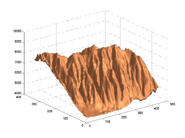
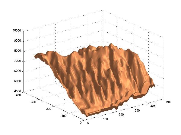
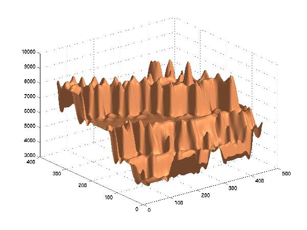
Here are the surfaces at various compression levels, plotted in 3D by Matlab.

Original

Lossy Compression to 1 Bit/Point, RMSE=6.0 meters
Lossy Compression to 0.1 Bit/Point, RMSE=51.7 m
Lossy Compression to 0.03 Bit/Point, RMSE=148 m
Lossy Compression to 0.01 Bit/Point, RMSE=535
The approximation shows the general aspect of the surface even down at 0.1 BPP, which is a compression by a factor of at least 100 compared to the original data. At 0.03 BPP, the original surface is still discernable, but serious artifacts appear.
Interpolating from contour lines to an elevation array is a classic problem in computational cartography. First, there are the traditional heuristics, such as extending straight lines in eight directions from the test point until they intersect eight contour lines, then interpolating with a weighted average, as described in Douglas (1983) and, later, Jones, el al (1986). Similar inverse-distance weighting methods are shown in Watson (1992) and Heine (1986), often using natural neighbors found by Sibson (1981). These methods can work if the contours are not kidney-shaped.
However, an artifact appears when interpolating a concentric set of circular contour lines, representing a cone. Since the outer contour line are longer than the inner ones, the averaging rule causes the surface between two contour lines to droop, as if pulled down by gravity, in an unaceptable scalloping or terracing effect. For a thin-plate interpolation, this effect is shown in Figures~\ref{f:figures/crater_beta} and \ref{f:figures/tuckermans_beta}.
Partial differential equations (PDEs) can be used to model a surface subject to certain constraints. Good cartographic introductions to PDEs for interpolation are Tobler (1979, 1986). One simple PDE is the Laplacian, or heat-flow equation,
where
etc. The relevance to heat-flow is that, if we map elevations to temperatures, assume that the contour lines are fixed at known temperatures, and assume that the surface conducts heat uniformly, then each point on the surface between the contour lines will eventually equilibrate to some temperature, which we map back to elevation. If this equation is solved by iteration on a grid, then the elevation of each point in the array, whose height is not already fixed, is the average of its four neighbors:
However, the Laplacian also demonstrates the terracing artifact.
The more complicated thin plate model minimizes total curvature, similar to fitting a thin sheet of metal to fixed points, while minimizing the energy of bending. Gaussian curvature, commonly used in geometry, is inappropriate here, since it is zero on a ``developable'' surface, such as a bent sheet of paper. Instead we use the (scaled) divergence, or
for the curvature at a point.
The partial differential equation is:
while the corresponding iterative equation on a grid is:
With this equation, information flows across the contour lines, which is desirable. This method produces less terracing, but instead demonstrates a ringing effect, similar to a Gibbs phenomenon when a square wave curve is being approximated by a Fourier series. Intuitively, the surface tries so hard to minimize the curvature, that, when the data is too nonsmooth, the surface has synthetic oscillations. For example, an interpolation of the desert floor next to a mesa would have this undesirable artifact.
Until a useful formal model of terrain elevation is available, the desirable characteristics of an interpolation or approximation algorithm are not obvious, since different attributes conflict with each other. For example, since geological features are stretched and distorted, an interpolation that is invariant with respect to nonuniform scaling in x and y might be desirable. However, this is not compatible with any algorithm using nearest points, such as a Voronoi method. Even allowing uniform scaling is incompatible with any algorithm containing an embedded constant distance, such as kriging. Again, second-degree continuity might be a desirable attribute, except that the real world is often not continuous at all. Forcing high-order continuity here will only create false ripples.
The conclusion is that visual inspection may be the best judge of an interpolation or approximation method. We may not be able to formalize it, but we know a good surface when we see one. In particular, we can easily see non-local artifacts, such as the terracing.
The following figure shows terracing and ringing schematically. The circles are the data points; the thin lines the interpolated surface.
Figure: Terracing and Ringing in an Interpolated Surface
If the input data is not exact, then interpolating it, exactly, may be the wrong operation. Instead, an approximate surface, which passes near the data, might be preferable, since it can have other desirable properties, such as virtually eliminating ringing. This can be realized by assuming that there are springs between the data points and the surface, and minimizing the total energy of the springs and the curvature, as done by Terzopoulos (1988). Unfortunately, the terracing is only reduced.
Explicitly solving a PDE on an NxN grid, without utilizing the system's sparsity, takes time N6, which is infeasible for large N. Sparse system solvers and iterative methods are more practical; their time is proportional to the desired accuracy. The best current iterative method is the multigrid. It finds an approximate solution on a coarse grid, then improves the solution on a finer grid, with periodic recourse back to the coarser grid for speed. The multigrid technique can solve systems with more than 10000x10000 cells. Terzopoulos (1983) used this method for solving the thin-plate equation. Douglas (1997) points to tutorials, bibliographies, and software on multigrids.
Voronoi interpolation of the data points is a completely different method, Gold & Roos (1994). Here, a Voronoi diagram is formed from the data points. The test point is inserted into the diagram, and the areas its Voronoi polygon steals from its neighbors are used to weight the neighbors' elevations. A Hermite transformation of the weights may be used to increase the continuity. Voronoi interpolation solves the problem of artifacts such as surface, slope, or curvatures discontinuities, slope or curvature discontinuities, and and local elevation extrema. Another promising idea is to use terrain-specific criteria and geomorphological rules to fit a Bezier surface, Schneider (1998). Carrara et al (1997) find that TIN and grid interpolation methods produce surfaces reflecting the ground morphology.
Triangulating the points into a Triangulated Irregular Network, perhaps with a Delauney triangulation, is a related method, Garcia (1992). Any interpolation method, either bilinear or a higher order spline, may be used inside each triangle. However, sometimes a triangle will have all three vertices on the same contour, causing it to be horizontal, which is undesirable. Christensen (1987) triangulates closed contour lines to create new elevation lines between existing contours. Rather than depicting the final surfaces, the paper shows the interpolated contours, on small, optimal, data sets.
Because linear interpolation may result in surfaces with flat areas, Watson (1992) blends the technique with a gradient estimation. Huber (1995) detects features such as ridges and valleys, interpolates new elevations on them, and then applies any other method to this enhanced set. This considerably reduces artifacts.
Their limits are
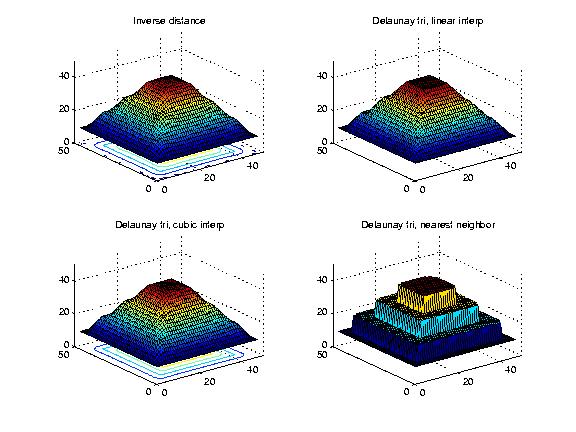
Figure: Interpolating 3 Nested Squares with Inverse Distance Weighting, and 3 Ways with Delaunay Triangles
The following shows a vertical slice thru the interpolating surfaces. It runs thru opposite corners, the better to show any artifacts. The triangulated line shows the original points. The other lines show the cubic, inverse distance, linear, and nearest neighbor interpolations. We see that none of the interpolations is acceptable since all show where the original contours are.
Figure: Figure: Vertical Slice Thru Four Interpolating Surfaces
Desirable properties include:
The new methods described here are based on the PhD work of Gousie (1998).
Our first new method repeatedly interpolates new contour lines between the original ones, somewhat similar to the medial axis. If two adjacent contour lines are: A, at elevation a, and B, at b, then we interpolate at elevation (a+b) thus.
Our contrarian philosophy is that we don't find the elevation at certain points, but rather find points with a certain elevation.
Figure: Crater Lake: Original Contours and Intermediate Contour Interpolation
The Maximum Intermediate Contours (MIC) method iterates the process, filling ever-finer contours. Alternatively, we can find intermediate contours one or more times, then do a thin-plate, Hermite-spline the peaks, inverse-distance weight other small gaps, and Gaussian-smooth the surface.
This method answers the problem of the generated surfaces terracing between contour lines by importing the idea of lofting from CAGD. It proceeds as follows. Generate a first version of a surface by any method. Find its gradient lines. Note that, on each gradient line, we know only the elevations where it crosses the contours. Interpolate its elevations in-between. This process smooths the surface, while keeping the interpolation. Springs may be added to any method, producing an approximation.
The following figures show three approximation methods applied to a 900x900 piece of the Crater Lake DEM. The first shows the original contour lines, which are seen to be separated by many pixels, which makes the process harder. The next three show the classic thin plate, and our intermediate contour and gradient line techniques. We see that both our techniques are much smoother than the thin plate, and that the gradient method is best. Our longer papers quantify this, and show more examples.
|
Figure 6. Crater Lake: Original Contours |

Figure 7. Thin Plate Approx |
Figure 8. Intermediate Contour Approx |
Figure 9. Gradient Line Approx |
The problem with many existing methods is that no information flows across the contours. This causes terracing. Our solution is to make the known data points also be the average of their neighbors. The method is to assume that there are N2 unknowns; i.e., even the known points are unknown. There are now two types of equations. First, for all points:
Second, for the known points, we make an equation that they are equal to their known values:
Since there are now more equations than unknowns, none of the equations will be satisfied exactly. That is, no points will be exactly the average of their neighbors, and the known points will not be exactly their known values. If there are K points whose elevations we know, then there are N2+K equations for the N2 unknowns.
We then do a least-squares solution in Matlab, to give an approximate solution, rather than an interpolation. With a least-squares solution, scaling an equation up makes it more important. Let R be the relative weight of the average-value equations compared to the others. A lower R will cause a more accurate surface, while a higher R will cause a smoother surface. A little inaccuracy goes a long way towards smoothing the surface.
Here is a test case constructed to stress any contour interpolation algorithm. It consists of four concentric squares, at a distance of five from each other. The squares' sharp corners facilitate artifacts, while the large gap between adjacent contours allows interpolated surfaces to droop or terrace. Our intuition would desire that a square pyramid with triangular sides result. However, few algorithms are likely to produce such a surface with discontinuities in the slope.
The next figure shows the surfaces that do result. R is the relative weight of the average-value equations. The four subfigures in order are the original contours, and the approximated surfaces with R=0.1, 1.0, and 3.0.
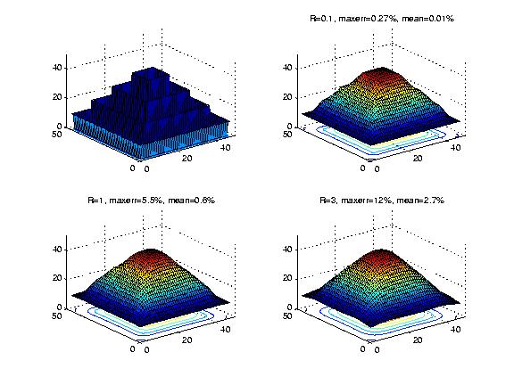
Figure: Overdetermined Laplacian PDE, Weighting Different Equations Differently
This figure shows the same four surfaces cut by a vertical plane cutting from corner to opposite corner, the better to show any artifacts. We see that with R=3, the location of the original contours is completely hidden, which is desirable.
Figure: Vertical Slice of the Surfaces
As the following table shows, the average error at the known points in this case is under 3%. That is, by allowing the elevations of known contour points to vary by an average of 3%, we can fit a quite smooth surface to the nested squares. Considering the accuracy standards of most hypsographic data, that may be acceptable.
| R | Max % Error | Mean % Error |
|---|---|---|
| 0.1 | 0.27 | 0.01 |
| 1.0 | 5.5 | 0.6 |
| 3.0 | 12 | 2.7 |
Note that our overdetermined solution concept is quite different from putting springs on the data points. That is also an approximation, but it does not try to make the data points to be the average of their neighbors. Absent that, it is impossible to make the surface not show the original contours.
Various extensions of the overdetermined solution technique are possible. We might calculate the error on each data point, then for the less-accurate points, increase their weights and re-solve. This reduces the max absolute error, but increases the mean. The resulting surface is slightly less smooth. Alternatively, we might guess that the points with large errors represent breaks in the surface slope. Then an reasonable response might be to reduce their weights and re-solve.
We have tested the overdetermined solution technique on grids of up to 257x257 points, and are working on larger cases.
Our proposed future work is follows. After adding splining to our TIN, and implementing a drainage basin routine, combine these various projects into a test suite, and test how well whether other terrain properties such as drainage patterns are preserved by these transformations. The goal is better to understand terrain with a view to formalizing a model of elevation.
This flow chart shows how the various parts can fit together.
Figure 11. Relations Among Our Research Components
Douglas, C. C. (1997), `MGNet', http://www.mgnet.org/.
Carrara, A., G. Bitelli, and R. Carla (1997), `Comparison of techniques for generating digital terrain models from contour lines', Int J Geographical Information Sciences 11(5), pp. 451-473.
Franklin, W. R. (1973), `Triangulated irregular network program', ftp://ftp.cs.rpi.edu/pub/franklin/tin73.tar.gz.
Franklin, W. R. (1994), `Triangulated irregular network program', ftp://ftp.cs.rpi.edu/pub/franklin/tin.tar.gz.
Franklin, W. R. & Ray, C. (1994), Higher isn't necessarily better: Visibility algorithms and experiments, in T. C. Waugh & R. G. Healey, eds, `Advances in GIS Research: Sixth International Symposium on Spatial Data Handling', Taylor & Francis, Edinburgh, pp. 751-770.
Franklin, W. R. & Said, A. (1996), Lossy compression of elevation data, in `Seventh International Symposium on Spatial Data Handling', Delft.
Garcia, Antonio Bello, e. a. (1992), A contour line based triangulating algorithm, in P. Bresnahan, E. Corwin & D. Cowen, eds, `Proceedings of the 5th International Symposium on Spatial Data Handling', Vol. 2, IGU Commission of GIS, Charleston SC USA, pp. 411-423.
Gold, C. M. & Roos, T. (1994), Surface modelling with guaranteed consistency -- an object-based approach, in T. Roos, ed., `IGIS'94: Geographic Information Systems', Lecture Notes in Computer Science No. 884, Springer-Verlag, pp. 70-87. http://www.gmt.ulaval.ca/homepages/gold/papers/ascona.html.
Gousie, M. B. (1998), Contours to Digital Elevation Models: Grid-Based Surface Reconstruction Methods, PhD thesis, Electrical, Computer, and Systems Engineering Dept., Rensselaer Polytechnic Institute.
Heine III, G. W. (1986), `A controlled study of some two-dimensional interpolation methods', Computer Oriented Geological Society Computer Contributions 2(2), 60-72.
Huber, M. (1995), Contour-to-DEM a new algorithm for contour line interpolation, in `Proceedings of the JEC '95 on GIS'. http://lbdsun.epfl.ch/ huber/ctdjec.html.
Jones, T. A., Hamilton, D. E. & Johnson, C. R. ( 1986), Contouring Geologic Surfaces with the Computer, Van Norstand Reinhold Company Inc., New York.
Ray, C. K. (1994), Representing Visibility for Siting Problems, PhD thesis, Electrical, Computer, and Systems Engineering Dept., Rensselaer Polytechnic Institute.
Said, A. & Pearlman, W. A. (1993), Reversible image compression via multiresolution representation and predictive coding, in `Proceedings SPIE', Vol. 2094: Visual Commun. and Image Processing, pp. 664-674.
Schneider, B. (1998), Geomorphologically sound reconstruction of digital terrain surfaces from contours, in `Eighth International Symposium on Spatial Data Handling', Dept of Geography, Simon Fraser University, Burnaby, BC, Canada, Vancouver BC Canada, pp. 657-667.
Sibson, R. (1981), A brief description of natural neighbor interpolation, in Barnet, ed., `Interpreting Multivariate Data', Wiley, pp. 21-36.
Terzopoulos, D. (1983), `Multilevel computational processes for visual surface reconstruction', Computer Vision, Graphics, and Image Processing 24, 52-96.
Terzopoulos, D. (1988), `The computation of visible-surface representations', IEEE Transactions on Pattern Analysis and Machine Intelligence 10(4), 417-438.
Tobler, W. (1979), `Smooth pycnophylatic interpolation for geographic regions', J. Am. Stat. Assn. 74(367), 519-536.
Tobler, W. (1996), `Converting administrative data to a continuous field on a sphere', http://www.sbg.ac.at/geo/idrisi/GIS_Environmental_Modeling/sf_papers/to bler_waldo/tobler_waldo.html.
Watson, D. (1992), Contouring: A Guide to the Analysis and Display of Spatial Data, Pergammon Press.