(in WR Franklin → Research)
Note: This page, created in April 2007, does not contain our latest results. Nevertheless, it may be interesting.
- Geo Star April 2007 Review - excellent summary of the project so far.
Project Goals
These may be summarized as follows.
- Study alternate terrain representations that are more compact.
- Since the new representations will therefore be lossy, evaluate the size / quality tradeoffs.
- These new representations ought to make it easier to represent legal terrain than illegal terrain.
- We wish to process datasets up to 10000x10000 elevation posts.
- With these new representations, uncompression speed is more important than compression speed.
- The new representations are to be evaluated on metrics such as visibility and mobility.
Summary of Accomplishments and Status
We are proceeding with researching alternative, more compact, representations of elevation data. We are now combining the various representations for greater power. Our initial evaluations of our alternative representations use, in addition to RMS elevation error, the observer siting and visibility metric. We are starting to employ the mobility metric. Here are some sample results.
- Our incremental Triangulated Irregular Network (TIN) program can process a 10800x10800 array of posts in internal memory on a PC. The accuracy is impressive; one dataset uses only 157,735 triangles to represent the 11,664,000 posts to a 3% maximum elevation error.
- Our scooping representation processed the W111N31 cell with 7x7 linear scoops to an average elevation error of 0.1%, and maximum error of 2%.
- We represented one 3592x3592 dataset with 7x7 scoops, and then compared the joint viewsheds resulting from multiobserver siting on the original representation and the alternate. The error was only 6.5%.
- We tested another new representation, ODETLAP, on a 400x400 piece of the Lake Champlain W cell. After selecting every third post in each of X and Y, that is 1/9 of the points, and using ODETLAP to fit a surface to them, the error was only 0.9 meters, or 0.1% of the elevation range.
- We are combining TIN with ODETLAP, in order to capture the essence of a surface with very few points.
- We can use ODETLAP to fill in radius 40 circles of missing data, with excellent results.
Professional Personnel
Various personnel, ranging from faculty members to grad students and undergrad students, have worked on the project, including the following.
- Dr W. Randolph Franklin, Associate Professor, RPI, PhD (Applied Math, Harvard): Strategizing, managing, writing, prototype coding.
- Dr Caroline Westort, Research Assistant Professor, RPI, PhD (Geography, Zürich): Strategizing about scooping.
- Dr Frank Luk, Professor, RPI, PhD (Computer Science, Cornell): Numerical analysis advice. Prof Luk is a former chair of CS, and is an internationally renowned expert in Scientific Computation.
- Metin Inanc, Research Assistant and PhD candidate (RPI): Incremental TIN, using ODETLAP to fill in missing data holes, the scooping alternative terrain representation.
- Zhongyi Xie, Research Assistant and PhD candidate (RPI): Using ODETLAP to reconstruct a surface from the minimal number of points generated by a TIN.
- Dan Tracy: PhD candidate (RPI): SVD approximations, multiobserver siting, path planning.
- Jared Scheuer, junior: studied aspects of ODETLAP during summer 2005. He measured the accuracy of either subsampling the surface, or of having a region of missing data, and using this technique to fill in the missing data.
- Rositsa Tancheva, junior: researched non photorealistic rendering (NPR) in computer graphics, in order to apply that to terrain. This was exploratory work that might lead to another new representation.
- John Shermerhorn, junior: also looking at some terrain issues, such as creating a testbed in which we can try our ideas.
- Joe Roubal, ESRI: implementing the multiobserver siting toolkit in ArcGIS.
- Steve Martin, undergrad (RPI): working during summer 2006 on sculpting terrain for Prof Westort.
- COL Clark Ray, PhD, provided valuable advice while at the USMA West Point.
Test Datasets and Protocols
These experiments used the following test datasets:
- USGS Lake Champlain W 1° DEM, which has a good mix of mountains, including Mt Marcy (the NYS highpoint), lowlands, and Lake Champlain.
- Assorted DTED level 2 data.
Our several testing protocols operate as follows.
- Compute some property on the original terrain representation, which is a large matrix of elevation posts
- Compute that property again on the alternative representation, whether TIN, scooping, or ODETLAP.
- Measure the difference between the two representations.
- Evaluate various test datasets.
- Examine the tradeoff between the size of the dataset and its quality.
Some of the various test protocols are the following.
- Protocol 1: Elevation Testing. Here we measure both average absolute error and RMS error. The reason is that some representations do better at one than at the other. In addition, we examine the terrain to see if its features are captured. This is important but hard to quantify.
- Protocols 2-4: Visibility Testing. These contain various
levels of complexity:
- Evaluate differences in observer viewsheds.
- Evaluate the visibility index of every observer in the cell.
- Evaluate multiobserver siting quality.
- Protocol 2: Viewshed Testing, which proceeds as follows.
- Select values for the following parameters: Radius of interest, R, and observer and target heights, H.
- Compute the viewshed bitmaps of many observers on both the original and the alternative representations. We can do this fast even for large R.
- For some observer O, let Vo be its viewshed on the original, and Va be its viewshed computed on the alternative representation. Vo and Va are bitmaps (i.e., sets of target points visible by O). Report the size of the symmetric difference, |Vo-Va| + |Va-Vo|.
- Protocol 3: Visibility Index Testing:
- Consider each post in term as an observer.
- Compute its visibility index.
- Using Monte Carlo sampling, pick T random targets, compute their visibility, and report the fraction visible.
- Produce a map of all the visibility indexes.
- Compare the visibility index map of the original terrain representation to the map of the alternative representation.
- Protocol 4: Multiple Observer Siting Testing
- Site a set of observers, So, on the original terrain representation.
- Site a set of observers, Sa, on the alternative terrain representation.
- Transfer Sa to the original representation.
- Compare the quality of Sa to that of So.
Alternative Terrain Representations
Our alternative terrain representations are as follows.
- TIN
- Scooping
- ODETLAP
- Combinations of the above, e.g., ODETLAP uses TIN points.
It is important to note that good compression techniques are multistep. For instance, JPEG combines the following sequential steps:
- Rotate from the RGB colorspace to the YCrCb colorspace.
- Perform a discrete cosine transform.
- Perform a low-pass filter.
- Arithmetic encode the remaining coefficients.
Text compression, e.g. bzip2, performs the following steps in sequence.
- Run length encoding.
- Burrows-Wheeler transformation.
- Move to front.
- Another run length encoding.
- Arithmetic encoding.
Our ultimate recommendation may well be a combination of our various techniques, perhaps as follows:
- Reconstruct an approximate surface with scooping, or
- Select significant points with TIN.
- Smooth the surface with ODETLAP.
- Fill in any local minima with our fast connected component program. (This program designed to process 3D cubes of bits, up to 600x600x600 voxels, resulting from threshholding a CAT scan. However, it can process 2D datasets as a special case. For example, one 18573x19110 image took 25 CPU seconds to process on a 1600 MHz laptop.)
Note that the last two steps do not increase the information content of our representation. That is, if they are a fixed part of our reconstruction engine, having them operate adds zero bits to the representation of the terrain.
Some experiments were performed by Tracy to compress the terrain using the singular value decomposition (SVD.) Various methods of partitioning the terrain and performing an SVD on each partition were tested. The results were inferior to those of competing compression methods. However, the SVD may still be useful in combination with other compression methods, such as scooping.
TIN
Features
Our version is a progressive resolution method.
- The initial TIN is just two triangles partitioning the cell.
- At each step, the post whose elevation is vertically farthest from the triangle containing its projection onto the XY plane is inserted into the triangulation, splitting one triangle into three.
- Often that point lies on an edge of the triangulation. In that case, one triangle is degenerate.
- If the new point lies on the cell's border, then its triangle is split into only two triangles.
- If necessary, a few edges are flipped to maintain the triangulation as Delauney. If one of the new triangles is degenerate, then one of its edges will always be flipped, removing the degeneracy.
This progressive resolution property is not common to some other triangulation methods, which may process the whole set of points at once. Our method may be stopped when any precondition is met. Typical preconditions include the insertion of a predetermined number of points, or the attainment of a predetermined maximum absolute error.
The points that have been inserted at that time are, in some sense, the most important points in the surface. They may then be used by a successive process such as ODETLAP. Since this point may not be widely appreciated, Figure 1 shows an example constructed to be difficult. The test dataset contains two overlapping circular ridges with sharp tops, transected by a railroad embankment with vertical sides.

Difficult Test Dataset for TIN
Figure 2 shows the result of applying TIN until the maximum error is sufficiently small. Note how points are selected along the ridges and embankment sides, and how the edges align with these features and do not cross them. Figure 3 is an enlarged detail.
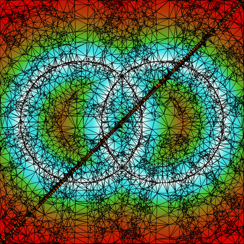
TIN of the Difficult Test
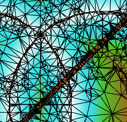
Detail of the TIN of the Difficult Test
The data structures used by our TIN method were the result of considerable thought before the first line of code was written. They are very compact, which is why we can process such large cells on a PC. For example, edges are not stored explicitly, but rather, each triangle has pointers to its (one to three) neighboring triangles. That saves space, at the cost of slowing down edge flips.
Feature points on the peaks and ridgelines, and the edges joining them, may be more important properties of the surface. Our TIN program selects them automatically; there is no need for manual identification and constrained triangulation. The points selected for the triangulation are assumed to be important, and can be fed into other methods, like ODETLAP. TIN is a piecewise linear triangular spline. Preliminary experiments with a higher degree spline showed no consistent improvement, and so were suspended.
Improvements This Year
Inanc modularized the TIN program and changed it in several ways. The error handling was changed to use C++'s exception handling mechanism. The code in the main() was removed and a new function was created to include the meta tasks for tinning. The Boost library's arrays were used for output.
Preliminary Testbed
A testbed using Python and the windowing library WXWin, (WXWidgets) was attempted. It was observed that the WXWin bindings (WXWin is a C++ library) for Python are not very stable. A side product was a GUI for the tinning program. The experimental testbed has a sluggish UI which is connected to a couple of C++ modules used to tin DEMs, render DEM files and render resulting TINs. A new testbed implementation is being built using Java, backed up by Matlab. This is justified by the fact that Java classes can be used natively within Matlab (Matlab's own GUI is Java based) and Java provides a rich set of libraries for building GUI and for scientific tasks. The new testbed is scooping/segmentation oriented.
Status
We can process 10800x10800 arrays of posts in 1/2 hour on a PC. No external storage is used. Our test dataset was formed by catenating nine 3601x3601 cells of data from the Savannah March kickoff meeting.
The elevation range of the dataset is 3600. TINning it until the maximum absolute error was 100, i.e., 3%, produced 157,735 triangles in 1292 CPU seconds. TINning it until the maximum absolute error was 10, i.e., 0.3%, produced 5.320,089 triangles in 1638 CPU seconds.
Lossless TIN
TIN is inherently lossy, but we can make it lossless as follows.
- Fit a surface to the TIN points, using any method.
- Compute the errors.
- Compress tue errors, say with PAQ3N.
The more TIN points that are used, the more accurate the reconstructed lossy surface will be, and the less space will be needed to code the errors. The goal is to minimize the sum of the two sizes. Figure 4 shows the tradeoff when using the Laplacian PDE to interpolate the points. Other methods, such as ODETLAP, would be better.
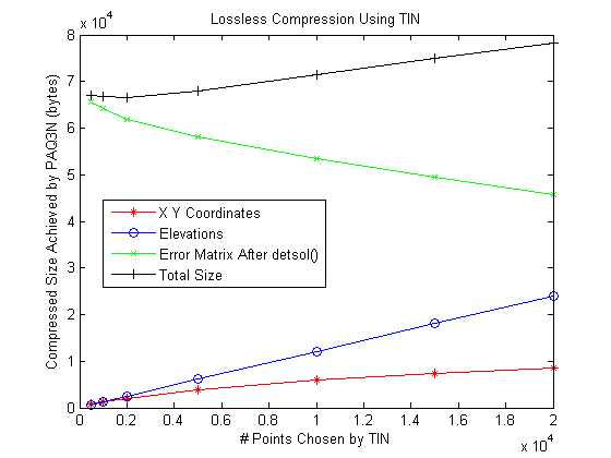
Tradeoffs with Lossless Compression with TIN
The (x,y,z) TIN points must finally be coded. In this, note that the order of the set elements is immaterial. Bitmap coding techniques suffice for (x,y). Assuming that there is not structure and that the points are random, there is an information theoretic limit. The coding of the (x,y) now determines the order of the zs. They may be compressed with a sequence of Burrow Wheeler, run length and arithmetic coding.
Scooping
This representation is longterm research. The goal is to smash through the information theoretic barrier to terrain compression by utilizing geologic information. We are pursuing several representations in parallel.
Several different shaped scoops were tried by Inanc. The most primitive scoops are flat-bottom scoops (0-degree equations). They are very effective in representing areas like seas, oceans, lakes, plateaus and any naturally occuring flat areas. In contrast, a Morse description is totally at loss with those structures. Our initial efforts concentrated on working with square shaped drills. The problem with those is that natural terrain does not segment easily into squares. Thus to represent a lake many square shaped scoops are required. An improvement was developing hierarchical scooping akin quad-tree representation. Thus if a single square is too big it will result in a representation error beyond a threshold and thus will be subdivided internally into smaller squares. To decrease the number of scoops more elaborate models were tried. 1-degree scoops are still flat, however a full blown planes which can be tilted to represent slopes. 2-degree scoops use quadratic equations and are still more versatile. 3-degree scoops (cubics) use prohibitively many parameters (10 coefficients). However with the increase of the degree of scoops the number of scoop applications required to represent the terrain accurately decreases.
A next and natural step is to build a segmentation algorithm which can take care of the natural shapes of geological formations. A constructive algorithm for segmentation can start by growing segments around seeds of initially selected points. If a point coincides with a lake the segment can be expected to grow to the full lake size merging other segments thus representing the whole lake with a single 0-degree flat-bottom scoop. The problem here is representing shapes. There are different ways to represent 2D shapes. The simplest way is to use bitmaps. Those can be compressed using fax compression algorithms. More complicated methods use Voronoi diagrams and build a skeleton to represent shape.
Some of the tests will now be described in more detail.
Degree-0 Scoops
The purpose of this was to learn what types of drills are more useful by implementing a Matlab test program. It is a greedy optimization - at each step, select the drill instance and location
(drill type, x, y, z)
that removes the most material. Drill instances will generally overlap. If two drills drill the same post, then the minimum elevation is used. This nonlinearity is radically different from, and more powerful than, wavelets. This nonlinearity also matches physical reality. If a river valley that cut 200' below the surrounding plane meets another river that is cut only 100' deep, then, at the confluence, the valley is only 200' deep, not 300'.
There are various subtleties of the greedy optimization. The drill that removes the most material at the start may be rendered completely redundant by later drills. This is reminiscent of stepwise multiple linear regression, where an initially important variable may ultimately be unimportant. A future possibility is to remove as well as add drills to the set. However this would be more compute intensive.
After the drills are determined, the final step would be encoding them. Note that the order of the drill applications is immaterial. Therefore, when coding, all the instances of the same drill may be grouped together. Then it is possible to sort the instances by location and delta encode the locations, since successive instances are relatively close. Alternatively a good bitmap compression method, such as CCITT group 4, could be used to code the drill locations.
The initial drills had no parameters other than their (x,y) location and (z) depth. One generalization, discussed in more detail later, is to allow more general (sloped) drills. This would tradeoff powerful, large to encode, basis elements, against small simple elements. However more of the simple more would be needed than of the complex ones. The sweet point would probably occur when the basis elements resemble the object being approximated. The purpose of these experiments is to better understand scooping, while initiating experiments in slope-preservation during lossy compression. The underlying assumption is that there is little long range correlation of elevation or slope.
An initial test on the 1201x1201 Lake Champlain West cell had these results. There were 11 drill types: a square of size 1 or 3, a circle of diameter 5, 10, or 20, a parabola of size 5, 10, or 20, and a flatter parabola of size 5, 10, or 20. After 10,000 drill instances, the initial material volume of 1.9x10⁹ was reduced to 4.2x10⁷. The mean absolute elevation among the 12012 posts was 30m, or 2% of the elevation range. 98% of the selected drill instances were the diameter 20 circle, with the diameter 10 circle and size 3 square distantly behind. The parabola drills were not selected even once. Table 1 gives the complete results.
| Drill Type | Count |
|---|---|
| Square, D=1 | 0 |
| Square, D=3 | 35 |
| Circle, D=5 | 2 |
| Circle, D=10 | 129 |
| Circle, D=20 | 9834 |
| Parabola, size 5 | 0 |
| Parabola, size 10 | 0 |
| Parabola, size 20 | 0 |
| Flatter parabola, size 5 | 0 |
| Flatter parabola, size 10 | 0 |
| Flatter parabola, size 20 | 0 |
We do not propose this specific set of drills as a polished technique to use, yet, but as an example of the experiments that we are conducting in order better to understand this idea.
Degree-1 Scoop
This version differs in the following ways. Instead of a set of overlapping drills, selected in a greedy manner, here there is only one drill, a 7x7 square, and the footprints of its applications partition the dataset. The face of each scoop is a tilted plane whose slope is chosen to minimize the elevation error.
Therefore, a 7x7 Scoop size represents 49 elevations using only 3 coefficients. 7 is not a magic number, and indeed we have experimented with various sizes. However, 7 is good enough for Level 2 DTED cells Large errors are rare and the mean error is very low, often less than 2 meters. The regularity brings simplicity to this representation.
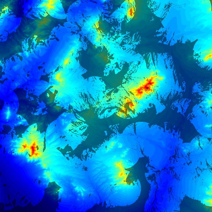
Here are some test results on the W111N31 DTED II cell, shown in Figure 5, with about 36002 posts with elevations from 811 to 2882, shown below. (To simplify the programming in these experiments, a few rows and columns were shaved off the sides of the cell to make the size an exact multiple of the tile size.)
W111N31 Cell
Figure 6 shows the effect of using fewer and larger tiles to approximate the cell. Even with 7x7 tiles, about 90% of the posts are represented to an absolute error under 4, or 0.2% of the elevation range.
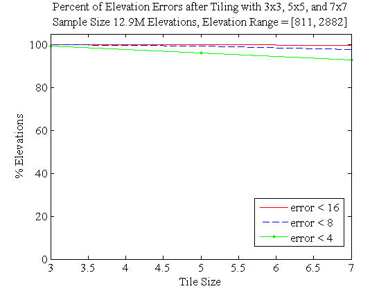
Percent of Posts with Errors Under Certain Cutoffs When Cell Approximated with Tiles of Various Sizes
Another test was performed with 5x5 drills, optimized with Singular Value Decomposition (SVD), on the Lake Champlain West cell, with a data range of 1576. The maximum error was 101, but that was rare. Over 50% of elevation posts were exactly represented. (This was helped by Lake Champlain being large and flat.) The input data size was 1442401 numbers, and the output data size 172800 numbers, for a compression ratio of 8.35:1. The contour images in Figure 7 contrast the original and reconstructed terrain. We see no visible difference.
Lake Champlain W Cell: Original and Represented by 5x5 Drills (Data Reduction Factor 8.35)
For another example, we used 7x7 drills to represent a 100x100 detail of the W111N31 cell, with an elevation range of 512. The reduction in data size is a factor of 16.3:1. Figure 8 shows the error histogram.
Next, we used observer viewsheds to evaluate this representation, as follows.
- Pick 81 observers,
- Assume that each observer is elevated 10 units above the terrain elevation at its location.
- Assume that each observer can see out to a radius of interest that is 300 posts.
- Assume that potential targets are also 10 units above their local terrain.
- For each observer, compute its viewshed, or what posts it can see, on the original dataset.
- Redo the computations on terrain reconstructed with the alternate representation.
- Measure the area of the symmetric difference between the two sets of viewsheds, as a fraction of the cell's area.
| Representation | % Error |
|---|---|
| tile3 | 1.31% |
| tile5 | 3.67% |
| tile7 | 6.52% |
| tile75 | 5.62% |
The tile3 representation approximates the surface with a regular grid of 3x3 tiles. tile5 and tile7 are similar. The tile75 representation uses first 7x7 and the 5x5 tiles.
Figure 8 and Figure 9 compare the joint viewsheds for the original terrain and the tile7 representation. The visible difference is small.
Sculpting
This is an extension of scooping being studied by Westort. She adapted a generic DTM sculpting tool definition and implementation from Java and C++ to Matlab, including blade, path, and target model matrices. With the help of Tracy and Luk, she significantly improved the efficiency of the code for large datasets. She evaluated the use of Arc/Map drainage and slope functionality for adoption as paths and blades, respectively. Together with Steve Martin, she is developing a stand-alone hydrological modeling solution for path and blade generation for DTM compression and reconstruction.
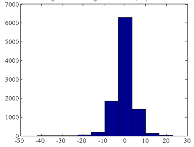
Error Histogram from Tiling 100x100 Detail of W111N31 with 7x7 Drills
Joint Viewsheds on the Original Terrain
Joint Viewsheds on the Tile7 Representation
This subproject has the largest potential payoff, for several
reasons. It will be able to represent discontinuities
(cliffs), and its nonlinearity is powerful. Dr Westort is
creating an initial testbed in Matlab to help us understand
the idea. This initial testbed will be of the nature of a
terrain reconstruction assistant. The user will specify the
terrain, the X-Y paths that the scoop (also called a blade)
will follow, and the blade's circular cross-section. The
system will run the blade along the path at the lowest
elevation that does not cut into the terrain. It will show the
error at each post and report the average and max error. We
anticipate demonstrating a prototype at the review meeting in
San Diego.
This testbed will provide a facility to gain experience with different blade shapes, including variable shapes. That experience will allow us to freeze some decisions, such as whether to use variable shapes, or not. The former choice will require fewer cutting paths, but with the latter choice, each path will take less space to represent. An analogy to splines would be, what is the appropriate polynomial degree to use?
Cutting paths are appropriate for canyon-like terrain. However, reconstructing, say, a mesa, might be better done with other operators. Designing such operators will be the next step, after we can reconstruct eroded terrain.
Postprocessing the reconstructed terrain with a smoothing operator might improve the accuracy at the cost of adding only one bit to the size of the representation ("apply the builtin smoother"). Smoothing will effective if the terrain satisfies some smoothness criterion, which contradicts our design principle that terrain is often discontinuous. Nevertheless, for completeness, this should be checked.
Finally, after obtaining a sufficient understanding of this idea, we might think about formulating and proving some theorems about it.
ODETLAP (Overdetermined Laplacian PDE)
This surface representation and reconstruction technique was pioneered by Franklin, and is being investigated in this project primarily by Xie. It extends the traditional Laplacian (heat flow) partial differential equation (PDE), which interplates unknown points in a matrix of known and unknown elevation posts, as follows. A system of linear equations is constructed with one equation for each unknown elevation, except those in the first or last row or column of the matrix:
4zij = zi-1,j + zi+1,j + zi,j-1 + zi,j+1
Choosing appropriate equations for the unknown border points is tricky, for some uninteresting technical reasons. The resulting sparse system easily can be solved by, e.g., Matlab, for 1201x1201 matrices. We call this technique DETLAP for exactly DETermined LAPlacian system. ODETLAP extends DETLAP as follows.
- One instance of the above equation is created for every (nonborder) point, whether known or unknown.
- Each known point also induces a second equation: zij = hij
- Each Border point induces a slightly different equation or two.
The resulting system of linear equations is overdetermined, i.e., inconsistent, so no exact solution is generally possible, but only a least square approximation, as follows. If the system is
Ax=b
we instead solve
Ax=b+e
so as to minimize the error e. The solution is
x = (AtA)-1Atb
The two types of equations may be given different relative weights, depending on the relative importance of accuracy versus smoothness. Matlab easily processes 400x400 matrices of elevation posts. More specialized techniqes can handle larger systems. See [^John Childs masters, A Two-Level Iterative Computational Method for Solution of the Franklin Approximation Algorithm for the Interpolation of Large Contour Line Data Sets, http://www.terrainmap.com/ ^], which uses a Paige-Saunders conjugate gradient solver with a Laplacian central difference approximation solver for the initial estimate.
ODETLAP has many advantages, which are not, to our knowledge, combined in any other surface approximation technique.
- It will infer a local maximum, i.e., a mountain top, inside a set of nested contours. Therefore, it does not generate artificial buttes all the time. This property can be surprising because points interpolated with a Laplacian PDE must fall inside the range of boundary value points. However, we're not doing an exact Laplacian PDE, but an extension of it. Therefore, we can generate values outside the range of boundary value points.
- The generated surface doesn't droop between contours. For reasonable weighting parameters, the contours are invisible in the resulting surface.
- It will utilize isolated data points, if available.
- If will interpolate broken contours. This is not a property of methods that fire out lines until they hit a contour.
- The resulting surface is at least approximately conformal. That is, if a conformal mapping is applied to the input points the resulting surface is that conformal map of the surface computed from the untransformed points. Therefore, sets of nested kidney-bean contours are handled reasonably. Again, this property is not shared by all surface approximation methods.
- ODETLAP will conflate inconsistent data, with user-defined weights, producing one merged surface. This allows one to combine a large, low-resolution dataset with one or more small high-resolution datasets covering only parts of the large dataset.
Figure 11 shows a stress test of ODETLAP. The test data is a set of four nested square contours. A surface is fit to them with ODETLAP run three times with different values of the smoothness parameter, R. Larger values for R mean a smoother but less accurate surface. The surfaces are plotted with an oblique projection so that the silhouette edge is obvious. The lower right surface shows no evidence at all of the original square contours, and interpolates a smooth moutain top in the center. The maximum absolute elevation error is 12% of the elevation range, and the mean only 2.7%. These errors would be much smaller for smoother contours.
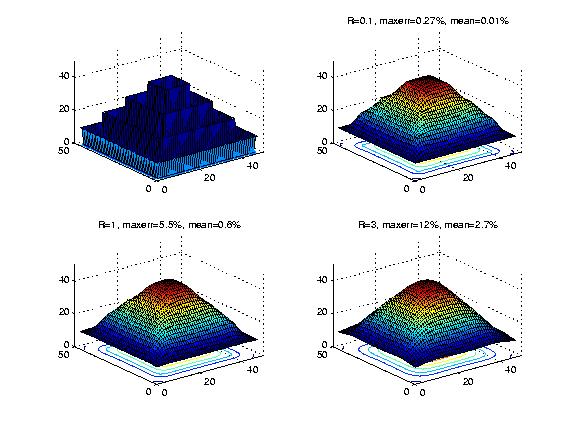
Nested Square Contours Generating Three ODETLAP Surfaces with Varying Smoothness and Accuracy
The impact of ODETLAP for this project is that surprisingly
few points are needed to generate a good surface.
We tested ODETLAP on a mountainous 400x400 section of the Lake Champlain W DEM, with elevation range 1378m, by selecting every Kth post in both directions and using ODETLAP to fit a surface (with R=0.1). The following table show that average absolute errors. Data set size % is the ratio of posts used to reconstruct the ODETLAP surface compared to the original number. It is 1/K2.
| K | Data set size, % | Error | Error % |
|---|---|---|---|
| 3 | 11.1% | 0.9 | 0.065% |
| 4 | 6.25% | 1.6 | 0.11% |
| 5 | 4% | 2.4 | 0.17% |
| 7 | 2% | 4.1 | 0.29% |
| 10 | 1% | 6.5 | 0.46% |
| 15 | 0.44% | 10 | 0.71% |
| 20 | 0.25% | 12 | 0.86% |
| 30 | 0.11% | 14 | 1.0% |
| 50 | 0.05% | 16 | 1.1% |
That is, with ODETLAP we reduced the data size by a factor of 100, at a cost of an average error of 0.46%
Choices for Input Points
Xie has have been mainly working on ODETLAP in the past year. To be more specific, he is trying different sampling methods on some 400x400 elevation matrices and then using ODETLAP to reconstruct the surface.
We have tried three different sampling methods.
- The first technique, the regular method is just regular sampling, i.e., choosing 1 point for each K points in both horizontal and vertical directions. The compression ratio is 1/K2.
- The second technique, the TIN method, is to use output points from the TIN program, which iteratively selects points furthest from the current surface.
- The third technique, the improved TIN method, operates
as follows.
- Run TIN to produce a predetermined number of important points.
- Use ODETLAP to reconstruct the surface from those points. Note that the surface will pass near, but not exactly through, the points.
- Find the worst points in that surface, that is the points whose reconstruction is farthest from their correct value.
- Add those points to the set of points from TIN, and rerun ODETLAP to compute a better surface.
Here is a comparison of the three methods on three 400x400 test cells, with ODETLAP smoothness parameter R=0.3. Both the regular and TIN methods used 1000 points. The refined TIN method added the 100 worst points from the TIN method. For each test, we measured the average absolute error and the maximum absolute error. The column headings are as follows.
| Abbrev | Meaning |
|---|---|
| TIN a | TIN, average error |
| Reg a | Regular, average error |
| Ref a | Refined TIN, average error |
| TIN m | TIN, max error |
| Reg m | Regular, max error |
| Ref m | Refined TIN, max error |
| Data | Reg a | TIN a | Ref a | Reg m | TIN m | Ref m |
|---|---|---|---|---|---|---|
| W111N3110 | 3.4 | 5.6 | 5.3 | 98 | 31 | 27 |
| W111N3111 | 9.0 | 10.6 | 10.4 | 134 | 113 | 66 |
| W111N3112 | 1.7 | 2.7 | 2.6 | 114 | 20 | 16 |
The TIN method produced a somewhat worse average error, but a much better maximum error. That is, the TIN method produced a much better conditioned surface. The refined method was slightly better then the TIN method under both the average and maximum metrics. Modifying the refined method to add even more bad points would presumably make it even better. That is an area for future research.
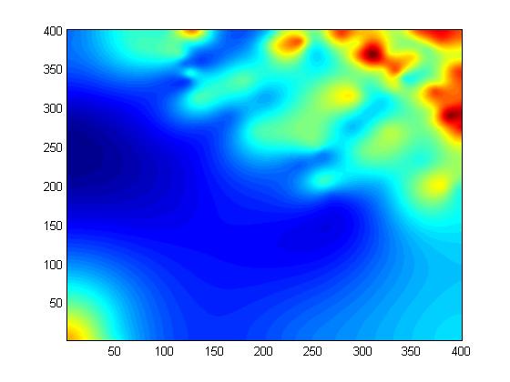
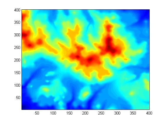
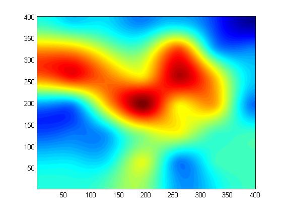
Figures 12 to 14 compare the regular and TIN methods, each with 100 points, on the W111N3110 dataset. Note how the TIN method captures small features better. Note also how well even 100 points represent the original surface.
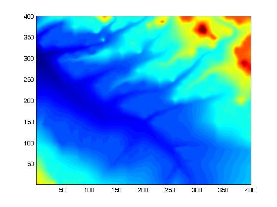
Original W111N3110 Dataset (160,000 Points)
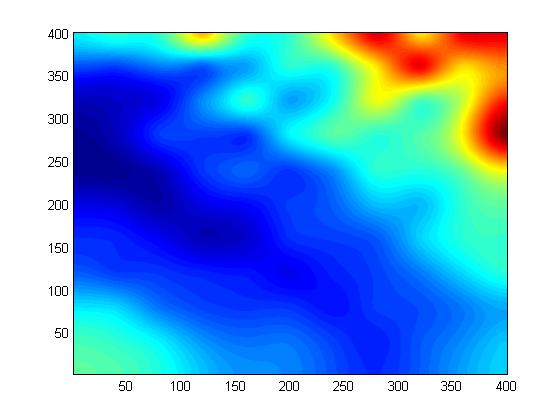
ODETLAP Fit to 100 Regular Points
ODETLAP Fit to 100 TIN Points
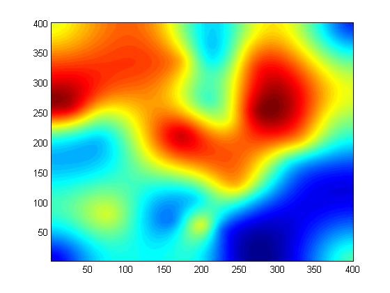
Figures 15 to 17 show an example of approximating a more complex surface with fewer points. Even only 36 TIN points capture the broad essence of the surface.
Original W111N3111 Dataset (160,000 Points)
ODETLAP Fit to 36 Regular Points
ODETLAP Fit to 30 TIN Points
We have also done some preliminary experiments on a new
sampling method, namely, the visibility method. This method
fits a surface to the points of greatest visibility.
Filling in Missing Data Holes
This topic was pursued because of sponsor interest expressed at the review meetings.
Terrain (elevation) data sometimes has holes or regions of missing data, perhaps because of the production technology. This section compares some algorithms for filling in a circle of radius r=100 of missing data. This missing region is large enough to stress-test the various algorithms, most of which are unacceptably bad. Any algorithm that succeeds here can also handle smaller holes.
The two best algorithms, which produce realistic results, are a thin plate PDE, and an overdetermined Laplacian PDE. The thin plate PDE is faster, while the overdetermined Laplacian PDE may also be used to smooth known data.
The test data and environment are as follows.
- The terrain format is an array of elevations.
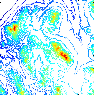
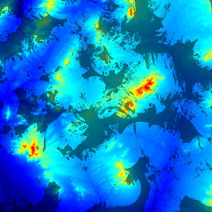
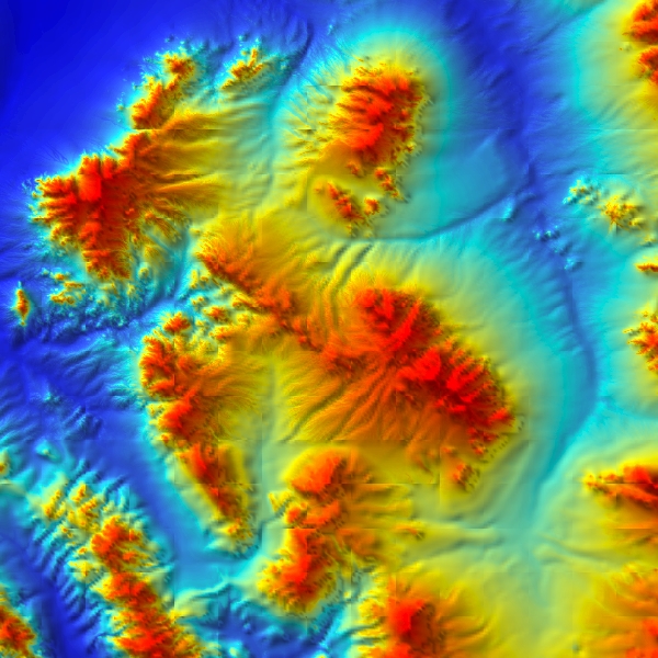
- The test data sets are drawn from the 1201x1201 Lake Champlain West USGS level 1 DEM, seen in Figure 18. It combines part of the Adirondack Mountains, the highest in NYS, with Lake Champlain and its lowlands. North is to the right.
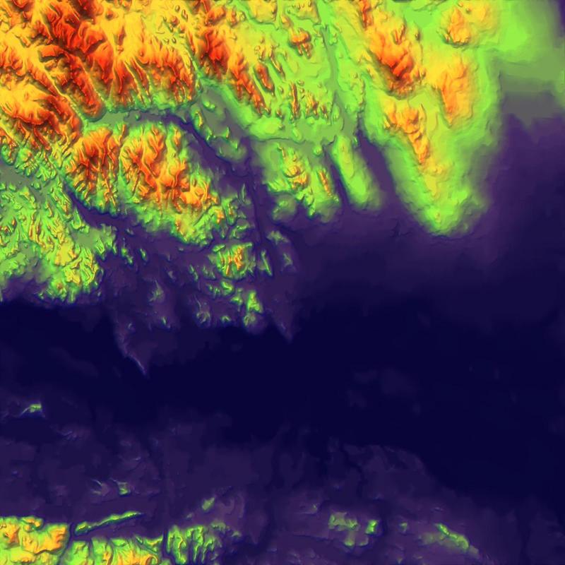
Lake Champlain West DEM
- The region of missing data, which needs to be interpolated, is always a circle of radius r=100.
- Each test missing circle was embedded in a 400x400 square of data. That is relevant only for the two interpolation algorithms that use data beyond the boundary of the missing data. Those are the two best algorithms, overdetermined Laplacian PDE and thin plate PDE. They actually use data within 2 posts of the circle of missing data. The poorer algorithms use only data on the circle.
Figure 19 nicely summarizes the results. The data outside the black circle (r=100) is real; the data inside was interpolated by our overdetermined Laplacian PDE. Although the thin plate PDE produces similar results, our method has other advantages that that lacks, such as the ability to conflate inconsistent data.
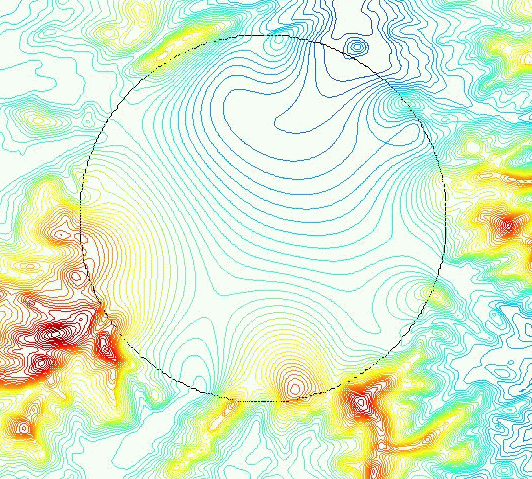
Using ODETLAP to Fill in the 31416 Missing Posts Inside the Circle
- Note the realistic appearance of the contour lines.
- Note the interpolated local mountain top near the bottom just inside the circle. That was caused by the large slope of the known terrain just outside the circle. This interpolated feature is remarkable since few interpolation algorithms can produce a value that is outside the range of the known values.
More detailed results are available at a web site with a javascript program allowing the user to choose from various preprocessed datasets, [^https://wrf.ecse.rpi.edu/Research/geostar-reports/fill_data_holes/index.html^]. That presents the results of 6 interpolation algorithms on 20 different sections of Lake Champlain West. Each cell of the table shows six algorithms on one dataset:
- R=.1 overdetsol()
- This is our overdetermined Laplacian PDE. R=.1 means that the equations for all points being equal to the average of their neighbors are weighted 0.1 as much as the equations for the known points being equal to their known values. That results in no visible smoothing of the known data.
- detsol()
- This is the Laplacian PDE for the unknown points.
- thinplate()
- This is the thin plate PDE for the unknown points.
- Matlab nearest
- This is the Matlab builtin nearest point interpolation algorithm, chosen because it is well known.
- Matlab linear
- This is the Matlab builtin linear interpolation algorithm.
- Matlab cubic
- This is the Matlab builtin cubic interpolation algorithm.
A fourth Matlab interpolation algorithm is not shown since it failed. Figure 20 compares the different techniques.
Comparing Six Methods to Fill in a Missing Data Hole
Planned future work on this topic is as follows.
- Using the builtin Matlab overdetermined linear equation solver for our overdetermined Laplacian algorithm is very slow. We are currently researching faster solution techniques.
- This algorithm can interpolate general classes of data, such as contour lines, possibly broken, and isolated points, perhaps derived from a TIN. We plan to study this in more detail.
Multiobserver Siting
This is prototype software originally written by Franklin, and extended Christian Vogt as a masters thesis. It is a set of C++ programs that exchange data in files and are controlled by Linux shell scripts and makefiles. The toolkit works, albeit being somewhat complicated and messy. It can quickly compute high resolution viewsheds as demonstrated in Figure 21.
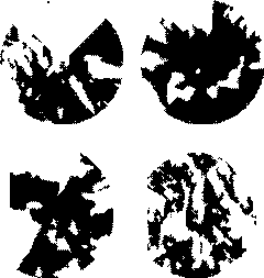
Sample Viewsheds
Dan Tracy is using the siting toolkit to evaluate our
compression. The following figures demonstrate the toolkit's
output. The test dataset is the Lake Champlain West DEM. A
particular radius of interest and observer and target height
are picked and the 60 observers are sited, so that their
viewsheds will jointly maximally cover the cell. See Figure
22. Figure 23 adds an
intervisibility requirement. That means that the
observers must form a connected graph, if there is a graph
edge between pairs of observers that can see each other. This
allows messages to be passed from observer to observer, which
is useful if they are radio base stations.
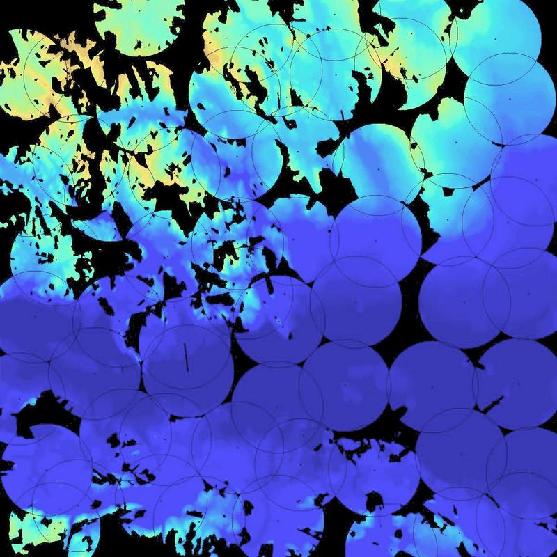
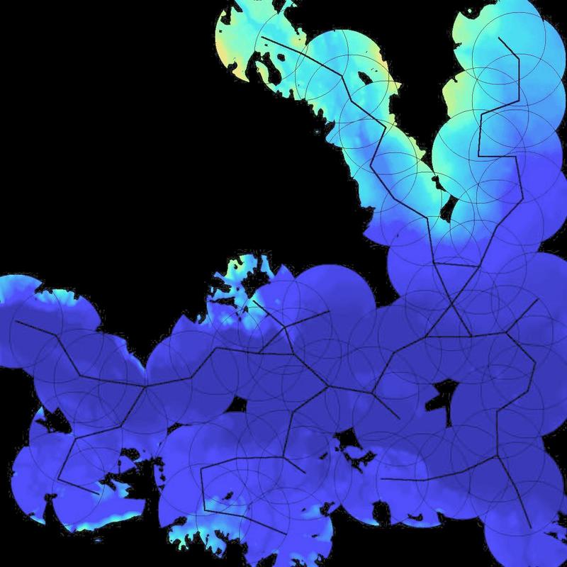
Siting 60 Observers on Lake Champlain W, WITH Intervisibility
Of course, the area of the joint viewshed is smaller since the
individual viewsheds must overlap, as quantified in Figure 24.
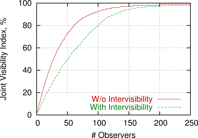
Effect on Joint Viewshed of Requiring Intervisibility as the Number of Observers is Increased
RPI has issued a subcontract to Environmental Systems Research
Institute, Inc. to productize our siting toolkit it as an
ArcGIS module. A copy of the contract was sent to DARPA/DSO
to check that the government will be able to use this module
for free.
Effect of Reducing Resolution
We earlier conducted initial studies of the effect of lowering the horizontal or vertical resolution of the dataset before performing the multiobserver siting. We observed that lowering the horizontal resolution lowers observer siting quality. However, lowering the vertical resolution does not have as large as effect.
The visibility, computed on the lower resolution data, is too high. In other words, when an observer's viewshed is computed on a lower resolution matrix of elevation posts, it may have a larger area (after scaling) than when computed on the original, high resolution, data. That means that it is important to compute the viewsheds on the best available data.
Careful consideration was given to the proper procedure for evaluating the effect of reduced resolution; the chosen procedure is given in below.
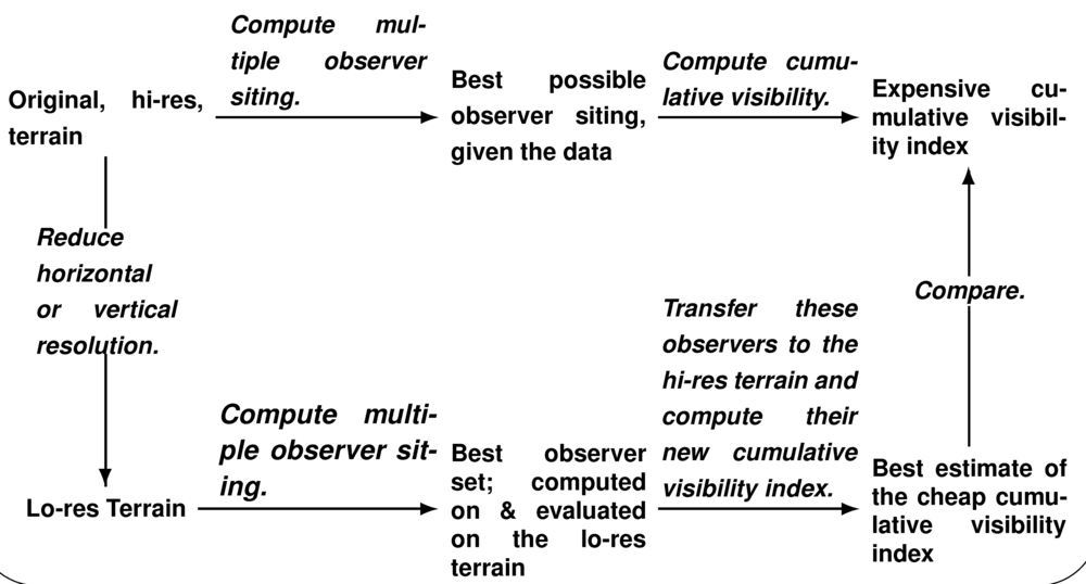
Reduced Resolution Evaluation Procedure
Our point is this. When evaluating a set of observers, it
does not matter where they are, but how much they can see.
There may be many sets of observers, each as good as the
other. Therefore, when performing a multiple observer siting
on the reduced resolution dataset, we compute their joint
viewshed, and compare its area to to that of the joint
viewshed of multiple observers sited on the original, best
quality, data. Also, when computing the viewshed area of the
observers sited on the lo-res data, we do the computation on
the hi-res data, since that is more accurate.
Figures 26 and 27 show some experiments with reducing the horizontal and vertical resolution. The visibility index is the fraction of the cell covered by the joint viewshed of a fixed number of observers sited with our testbed. The ''hi res'' line shows the result of using the original data. The lo-res line shows the siting and viewshed computation formed on the lo-res data, for three different reductions in horizontal resolution. The transferred res line shows the effect of siting the observers on the lo-res data, but then computing their joint viewshed on the hi-res data. It is this line that should be compared to the hi res line. The extent to which it is smaller shows the deleterious effect of reducing the data resolution.
The difference between the lo res and transferred res lines shows the error caused by evaluating viewsheds on lo-res data. That the lo res line is higher shows that the error is biassed up. There may be no deep significance to this; it may be an artifact of how we interpolate elevations between adjacent posts.
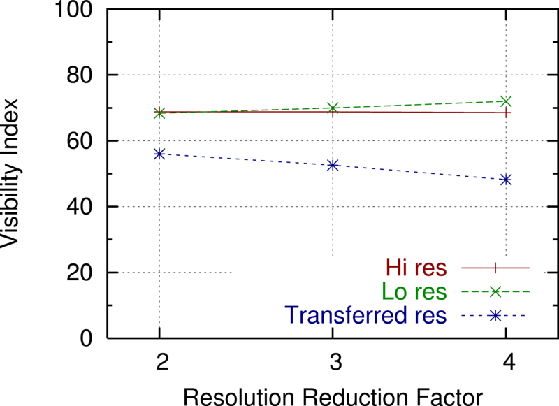
Effect of Reducing Horizontal Resolution on Visibility Computation
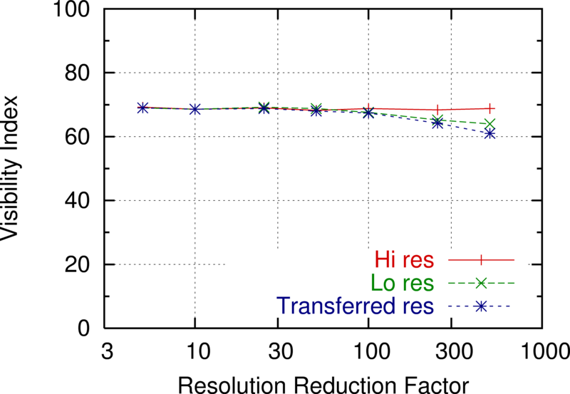
Effect of Reducing Vertical Resolution on Visibility Computation
Figure 28 shows how imprecise viewshed computations
can be. The test data is the Lake Champlain West cell; the
observer is near the lower left corner, on Mt Marcy. A
particular observer and target height are chosen, and then the
visibility of each point in the cell is computed by running
lines of sight from the observer. When the line runs between
two posts with elevations A and B, and some
elevation must be computed there, one of four rules is used.
- min(A,B)
- mean(A,B)
- linear interpolation between A and B depending on their relative distances from the line of sight.
- max(A,B)
The choice of interpolator affects the visibility of '''one half''' of all the points in the cell. The black region is hidden for all the interpolators. The dark grey region is hidden for three interpolators, the light grey region for one, and the saturated color region is visible for all of the interpolators. In other words, the visibility of (at least!) one half of the cell is actually unknown.
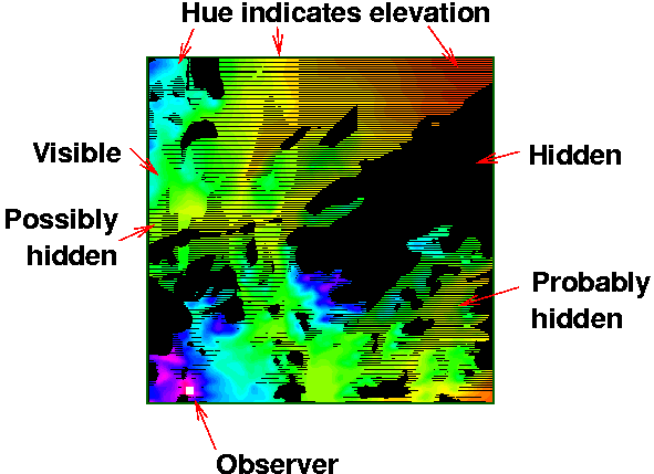
Viewshed Uncertainty Caused by Choice of LOS Elevation Interpolator
Smugglers' Path Planning
A path planning program was created by Tracy. Given a cost metric for the terrain, a start point, and an end point, the program computes the path between the two points that minimizes the line integral over the cost metric by implementing the A* algorithm. In particular, with a strictly binary go/no go cost metric (e.g. avoid the area visible by the planted observers,) the Euclidean distance of the path is minimized. We call this smugglers' path planning.
Future work may entail computing other error metrics related to the visibility and path planning.
Using Smugglers' Path Planning to Evaluate Alternate Representations
The purpose for researching alternate terrain representations is to use the terrain for some application, such as path planning. Since the alternate representation is good only so far as it supports such applications, we have started to use them to evaluate our representations, in addition to using elevation error.
The assumption is that the cost of a path between some source and goal depends on the how visible that path is to a set of observers. If our client is a smuggler, then low visibility is desirable. Conversely, if our client is using a radio and the observers are base stations, then high visibility is good.
Initially, we are computing paths that stay out of the joint viewshed of a set of observers optimally sited to see as much as possible of the terrain. Finding no suitable implemenation on the web, we implemented this ourselves. (The main difficulty is that the cost matrix is large and sparse. A second problem is that it is impossible explicitly to compute and store the distance between every pair of mutually visible points; remember that we are not working with toy-sized datasets.) Here is one test of our techniques.
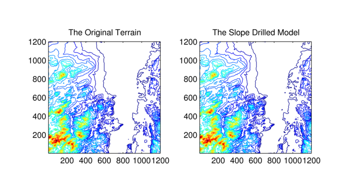
Figure 29 shows the test dataset, W111N31, 3595x2595 posts with 12,924,025 coefficients (elevations). The elevation range is 2071.
Smugglers' Path Planning Test Data
The alternate representation is to use 7x7 scoops. The
reduced the number of coefficients to 791,267, that is, by a
factor of 16:1. The mean absolute elevation error was 1.7, or
0.1%. There is no visible difference in the image of this
representation.
Next we optimally sited 324 observers, with radius of interest 100, to maximize their joint viewshed, shown in Figure 30.
Joint Viewshed of Optimally Sited Observers on the Tile7 Terrain Representation
Then we picked a source and goal that would have a complicated path between them, computed the shortest path that avoided the joint viewshed, and plotted the terrain, viewsheds, and path together in Figure 31.
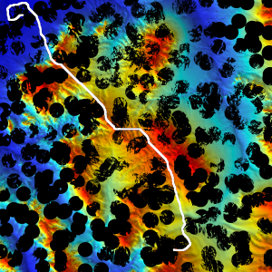
Shortest Smugglers' Path Computed Avoiding the Joint Viewshed
Our first evaluation of the alternate representation went as follows. We transferred the 324 observers back to the original terrain and recomputed their viewsheds. Then we overlaid the path on them and counted how many path pixels were inside the more accurate viewsheds. The path was 4767 points long; only 14, or 0.3% were visible, as shown in the Figure 32.
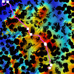
Undesirable Visible Path Points on Accurate Joint Viewshed
Coding the Representation's Coefficients
The representations discussed in this report all reduce the terrain to a set of coefficients. The raw dataset is a matrix of elevations. The degree-1 scoops are triples of coefficients of planes, and so on. As a final step, these coefficients must be coded, or reduced to a minimal number of bits. There is a wide range of coding research to draw on, such as JPEG when the coefficient matrix looks like an image. However, we hope to do better. This is future research.
Comparison of Actual Achievements with Goals
This project's progress is aligned with the proposal except for the following change. Because of sponsor feedback, we are researching path planning, instead of hydrology.
Cost Overruns
None.
Interactions Between RPI and Sponsors
In addition to written reports, there have been several face-to-face meetings during this contract.
- March 2005: kickoff meeting in Savannah GA, including presentation by WR Franklin.
- June 2005: site visit by Paul Salamonowicz and Ed Bosch of NGA to RPI.
- Nov 2005: Program review meeting in San Diego CA, including presentation by WR Franklin.
- April 2006: Program review meeting in Snoqualmie WA, including presentation by WR Franklin.
In addition, a password-protected website has been established, [^https://wrf.ecse.rpi.edu/pmwiki/GeoStar/^], to communicate results in a less formal manner.
Press and Blog Mentions
With the prior approval of DARPA, RPI announced the contract with a press release that was mentioned in the following RPI places.
- RPI Press release, 10/31/2005
- RPI School of Engineering Press Release
- Rensselaer School of Engineering News
- Improving Terrain Maps, Rensselaer Alumni Magazine Winter 2005-06
That press release was picked up by these news sources.
- Better terrain maps of Earth... and beyond, in Roland Piquepaille's Technology Trends, 5 nov 2005
- ZDNet, 11/5/2005
- Surfwax Government News
- Defence Talk, 11/1/2005
- Advanced Imaging (no longer online)
- ACM Technews 7(862), 11/2/2005
- Interview on WGY AM-810 radio, 11/3/2005
[^#^]
Papers and talks:
- bibtexsummary:[/wrf.bib,tracy-fwcg-2006]
- bibtexsummary:[/wrf.bib,inanc-fwcg-2006]
- "Computational and Geometric Cartography" presented at Siena College 22 Apr 2003 and Boston U 30 Apr 2003. Slides. (This is an updated version of my GIScience 2002 talk.)
- "Computational and Geometric Cartography", (invited keynote talk) GIScience 2002, Boulder, Colorado, USA, 26-29 Sept, 2002. Slides.
- Geospatial terrain: algorithms and representations, unpublished paper, and talk, April 2002. Abstract: Geospatial terrain elevation contains long-range, nonlinear relationships, such as drainage networks. Representations and operations, such as compression, that ignore this will be inefficient and possibly erroneous. For example, multiple correlated layers may become internally inconsistent. This paper presents various representations, and terrain operations (such as visibility), discusses criteria for a good representation, and attempts a start towards a formal mathematical foundation.
- "Mathematical Issues in Terrain Representation, presented at DARPA/NSF OPAAL Workshop and Final Program Review, 10 Jan 2002. Slides.
- H Pedrini, WR Schwartz, and WR Franklin. "Automatic Extraction of Topographic Features Using Adaptive Triangular Meshes, 2001 International Conference on Image Processing (ICIP-2001), Thessaloniki, Greece, 7-10 Oct 2001.
- bibtexsummary:[/wrf.bib,wrf-cagis-00] Paper. This was also presented as a talk on 20 April 2000. Abstract: Several applications of analytical cartography are presented. They include terrain visibility (including visibility indices, viewsheds, and intervisibility), map overlay (including solving roundoff errors with C++ class libraries and computing polygon areas from incomplete information), mobility, and interpolation and approximation of curves and of terrain (including curves and surfaces in CAD/CAM, smoothing terrains with overdetermined systems of equations, and drainage patterns). General themes become apparent, such as simplicity, robustness, and the tradeoff between different data types. Finally several future applications are discussed, such as the lossy compression of correlated layers, and just good enough computation when high precision is not justified.
- bibtexsummary:[/wrf.bib,wrf-ica99-web] Abstract: We describe several past and proposed projects for converting elevation data to different formats, such as gridded, TIN, and spline, lossily compressing, applying to visibility and drainage to test the compression quality, and integrating everything into a test suite. Our predominant elevation data structure is a grid (array) of elevations. We have also worked with a Triangulated Irregular Network (TIN), which the first author first implemented (under the direction of Poiker and Douglas) in 1973. This work has several themes, such as leveraging from recent results in applied math, skillfully implementing our algorithms, and testing them on realisticly large data sets. Efficient calculation of visibility information was one project. This includes determination of the the viewshed polygon of a specific point, or the visibility index of all points. The data processed includes several 1201x1201 level-1 DEMs and DTEDs. One surprise was that often there was no correlation between elevation and visibility index. Lossless and lossy compression of elevation data was another project. We used a wavelet-based technique on 24 random level-1 USGS DEMs. Lossless compression required 2.12 bits per point on average, with a range from 0.52 to 4.09. With lossy compression at a rate of 0.1 bits per point, the RMS elevation error averaged only 3 meters, and ranged from 0.25 to 15 meters. Even compressing down to 0.005 bits per point, or 902 bytes per cell, gave an indication of the surface's characteristics. This performance compares favorably to compressing with TINs. If it is desired to partition the cell into smaller blocks before compressing, then even 32 x 32 blocks work well for lossless compression. Approximating elevation data from contours to a grid is the latest project. Our first new method repeatedly interpolates new contour lines between the original ones. The second starts with any interpolated or approximated surface, determines its gradient lines, and does a Catmull-Rom spline interpolation along them to improve the elevations. We compare the new methods to a more classical thin-plate approximation on various data sets. The new methods appear visually smoother, with the undesirable terracing effect much reduced. The third new method is a realization of the classic proposals to use a partial differential equation (PDE) to interpolate or approximate the surface. Previously, this was possible only on small data sets. However, with recent sparse matrix and multigrid techniques, it is now feasible to solve a Lagrangian (heat flow) PDE on a 1000x1000 grid. It is also possible to solve an overdetermined system of equations for a best fit. Here, even the known points are constrained to be the average of their neighbors; so there are more equations than unknowns. This causes the slope to be continuous across the contours, and smooths the result. Our proposed future work is to combine these various projects into a test suite, and to test how well whether other terrain properties such as drainage patterns are preserved by these transformations. The goal is better to understand terrain with a view to formalizing a model of elevation. Slides.
- "Elevation data operations", ''Dagstuhl-Workshop on Computational Cartography'', (by invitation), Nov. 1996. Slides. Abstract: We describe several past and proposed projects for converting elevation data to different formats, such as gridded, TIN, and spline, lossily compressing, applying to visibility and drainage to test the compression quality, and integrating everything into a test suite.
- bibtexsummary:[/wrf.bib,wrflossy] Abstract: Generic lossy image compression algorithms, such as Said & Pearlman's, perform excellently on gridded terrain elevation data. We used 24 random 1201x1201 USGS DEMs as test data. Lossless compression required 2.12 bits per point on average, with a range from 0.52 to 4.09. With lossy compression at a rate of 0.1 bits per point, the RMS elevation error averaged only 3 meters, and ranged from 0.25 to 15 meters. Even compressing down to 0.005 bits per point, or 902 bytes per cell, gave an indication of the surface's characteristics. This performance compares favorably to compressing with Triangulated Irregular Networks. If it is desired to partition the cell into smaller blocks before compressing, then even 32x32 blocks work well for lossless compression. However, for lossy compression, specifying the same bit rate for each block is inadequate, since different blocks may have different elevation ranges. Finally, preliminary tests suggest that the visibility indices of the points are robust with respect to even a quite aggressive lossy compression.
- bibtexsummary:[/wrf.bib,wrfelev95] Abstract: This paper compares several, text and image, lossless and lossy, compression techniques for regular gridded elevation data, such as DEMs. Sp_compress and progcode, the best lossless methods average 2.0 bits per point on USGS DEMs, about half the size of gzipped files, and 6.2 bits per point on ETOPO5 samples. Lossy compression produces even smaller files at moderate error rates. Finally, some techniques for compressing TINs will be introduced. This paper is largely obsoleted by the first one listed above. However, this one also gives examples where partitioning the data before compressing generally does not increase the total compressed size, and suggests that that generally holds.